
Ficheiro:HittingTimes1.png

Dimensões desta antevisão: 800 × 600 píxeis. Outras resoluções: 320 × 240 píxeis | 640 × 480 píxeis | 1 024 × 768 píxeis | 1 200 × 900 píxeis.
Imagem numa resolução maior (1 200 × 900 píxeis, tamanho: 17 kB, tipo MIME: image/png)
|
|
Esta imagem provém do Wikimedia Commons, um acervo de conteúdo livre da Wikimedia Foundation que pode ser utilizado por outros projetos.
|
| Descrição |
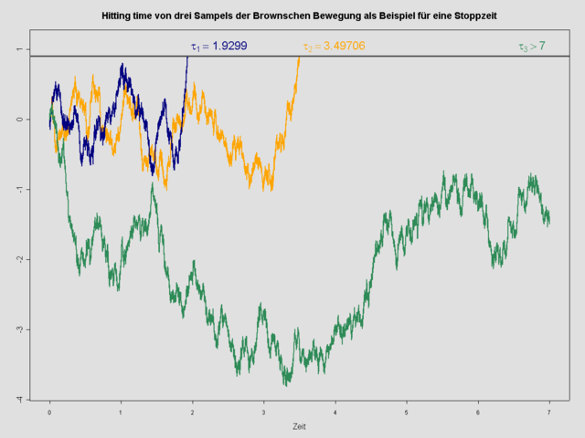
English: Hitting times and stopping times of three samples of brownian motion
Deutsch: Hitting time von drei Sampels der Brownschen Bewegung als Beispiel für eine Stoppzeit. |
| Data | |
| Origem | with the help of GNU R statistics / math software. see the source below |
| Autor | Thomas Steiner |
| Permissão (Reutilizar este ficheiro) |
Thomas Steiner put it under the GFDL |

|
Esta imagem de gráficos (ou todas as imagens neste artigo ou categoria) deveriam ser recriadas usando gráficos vectoriais, como ficheiros SVG. Isto tem várias vantagens; veja as Commons:Media for cleanup|imagens para rever para mais informações. Se já criou um ficheiro SVG desta imagem, por favor, carregue-o. Depois do novo ficheiro SVG ter sido carregado, substitua aqui esta predefinição pela predefinição {{vector version available|nome da nova imagem.svg}}.
|
(An SVG version should ideally not include the title text, which should be a separate caption as text instead to allow this to be useful in any language).

|
É concedida permissão para copiar, distribuir e/ou modificar este documento nos termos da Licença de Documentação Livre GNU, versão 1.2 ou qualquer versão posterior publicada pela Free Software Foundation; sem Secções Invariantes, sem textos de Capa e sem textos de Contra-Capa. É incluída uma cópia da licença na secção intitulada GNU Free Documentation License. |
| A utilização deste ficheiro é regulada nos termos da licença Creative Commons - Atribuição-CompartilhaIgual 3.0 Não Adaptada. | ||
| ||
| Esta marca de licenciamento foi adicionada a este ficheiro durante a atualização da licença GFDL. |
R-source code:
T=7
N=100000
set.seed(303898)
a=0.9
cs=c("orange", "navy", "seagreen4", "grey31")

bm1=c(0,cumsum(rnorm(N,mean=0,sd=sqrt(T/N))))
tau1=which(bm1>a)[1]
bm1[tau1:(N+1)]=a

bm2=c(0,cumsum(rnorm(N,mean=0,sd=sqrt(T/N))))
tau2=which(bm2>a)[1]
bm2[tau2:(N+1)]=a

bm3=c(0,cumsum(rnorm(N,mean=0,sd=sqrt(T/N))))
tau3=which(bm3>a)[1]
bm3[tau3:(N+1)]=a

png(filename = "HittingTimes1.png", width=1200, height=900, pointsize = 12)
par(bg="gray88")
t=seq(0,T,length=N+1)
plot(t,bm1,type="l",ylim=range(bm1,bm2,bm3,a*1.2),col=cs[1],lwd=2,ylab="",xlab="Zeit",main="Hitting time von drei Sampels der Brownschen Bewegung als Beispiel für eine Stoppzeit")
lines(t,bm2,col=cs[2],lwd=2)
lines(t,bm3,col=cs[3],lwd=2)
abline(h=a,col=cs[4],lty=1,lwd=3)

text(x=tau1*T/N,y=a*1.14, labels = substitute(tau[2]==t1,list(t1=tau1*T/N)),pos=4,col=cs[1],cex=1.5)
text(x=tau2*T/N,y=a*1.14, labels = substitute(tau[1]==t2,list(t2=tau2*T/N)),pos=4,col=cs[2],cex=1.5)
text(x=T,y=a*1.14, labels = substitute(tau[3]>T,list(T=T)),pos=2,col=cs[3],cex=1.5)
dev.off()
Histórico do ficheiro
Clique uma data e hora para ver o ficheiro tal como ele se encontrava nessa altura.
| Data e hora | Miniatura | Dimensões | Utilizador | Comentário | |
|---|---|---|---|---|---|
| atual | 23h03min de 7 de abril de 2006 | | 1 200 × 900 (17 kB) | Thire | |
| 22h53min de 7 de abril de 2006 |  | 1 200 × 900 (18 kB) | Thire | {{Information| |Description = some stopping times (even hitting times!) of brownian motion |Source = with the help of GNU R statistics / math software. see the source below |Date = 8 Apr. 2006 |Author = Thomas Steiner |Permission = |
Utilização local do ficheiro
As seguintes 2 páginas usam este ficheiro:
Utilização global do ficheiro
As seguintes wikis usam este ficheiro:
- ca.wikipedia.org
- de.wikipedia.org
- de.wikibooks.org
- en.wikipedia.org
- es.wikipedia.org
- fa.wikipedia.org
- fr.wikipedia.org
- it.wikipedia.org
- ko.wikipedia.org
- nl.wikipedia.org
- pl.wikipedia.org
- ru.wikipedia.org
- zh.wikipedia.org