Cálculo com múltiplas variáveis (também conhecido como cálculo multivariável ) é a extensão do cálculo em uma variável ao cálculo em diversas variáveis: as funções as quais são diferenciáveis e integráveis envolvem várias variáveis ao invés de uma única variável.
Não é mais que a extensão do cálculo infinitesimal a funções escalares e vetoriais de várias variáveis, com tudo o que esta generalização implica.
Campo escalar com duas variáveis. Cálculo diferencial em campos escalares e vetoriais [ editar | editar código-fonte ] Funções de Rn em Rm . Campos escalares e vetoriais [ editar | editar código-fonte ] Formulando as definições para campos vetoriais , estas também sendo válidas para campos escalares . Seja
f
:
V
⟶
W
{\displaystyle \mathbf {f} :V\longrightarrow W}
um campo vetorial que faz corresponder a todo ponto P definido biunivocamente por sua vetor posição um vetor
f
(
O
P
)
{\displaystyle \mathbf {f} {\big (}\mathbf {OP} {\big )}}
O é a origem de coordenadas .
V
⊆
R
n
,
W
⊆
R
m
,
{\displaystyle V\subseteq \mathbb {R} ^{n},W\subseteq \mathbb {R} ^{m},}
n
>
1
{\displaystyle n>1}
m
⩾
1
{\displaystyle m\geqslant 1}
m
=
1
{\displaystyle m=1}
campo escalar . Para
m
>
1
{\displaystyle m>1}
campo vetorial . Utiliza-se a norma euclidiana para encontrar a magnitude dos vetores .Sejam
a
∈
R
n
{\displaystyle \mathbf {a} \in \mathbb {R} ^{n}}
b
∈
R
m
.
{\displaystyle \mathbf {b} \in \mathbb {R} ^{m}.}
lim
x
→
a
f
(
x
)
=
b
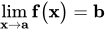
{\displaystyle \lim _{\mathbf {x} \to \mathbf {a} }\mathbf {f} {\big (}\mathbf {x} {\big )}=\mathbf {b} }
ou ainda,
f
(
x
)
→
b
{\displaystyle \mathbf {f} (\mathbf {x} )\rightarrow \mathbf {b} }
x
→
a
{\displaystyle \mathbf {x} \rightarrow \mathbf {a} }
para expressar o seguinte:
lim
‖
x
−
a
‖
→
0
‖
f
(
x
)
−
b
‖
=
0
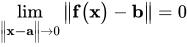
{\displaystyle \lim _{{\big \|}\mathbf {x-a} {\big \|}\to 0}{\big \|}\mathbf {f} {\big (}\mathbf {x} {\big )}-\mathbf {b} {\big \|}=0}
onde
‖
x
‖
{\displaystyle {\big \|}\mathbf {x} {\big \|}}
norma euclideana de
x
{\displaystyle \mathbf {x} }
Expresando-o em função das componentes de
x
=
(
x
1
,
…
,
x
n
)
,
a
=
(
a
1
,
…
,
a
n
)
,
{\displaystyle \mathbf {x} ={\big (}x_{1},\ldots ,x_{n}{\big )},\mathbf {a} ={\big (}a_{1},\ldots ,a_{n}{\big )},}
lim
(
x
1
,
…
,
x
n
)
→
(
a
1
,
…
,
a
n
)
f
(
x
1
,
…
,
x
n
)
=
b
{\displaystyle \lim _{{\big (}x_{1},\ldots ,x_{n}{\big )}\to {\big (}a_{1},\ldots ,a_{n}{\big )}}\mathbf {f} {\big (}x_{1},\ldots ,x_{n}{\big )}=\mathbf {b} }
ou, de forma equivalente,
lim
x
→
a
f
(
x
)
=
b
{\displaystyle \lim _{\mathbf {x} \to \mathbf {a} }\mathbf {f} {\big (}\mathbf {x} {\big )}=\mathbf {b} }
Dizemos que uma função
f
{\displaystyle \mathbf {f} }
contínua em
a
⇔
lim
x
→
a
f
(
x
)
=
f
(
a
)
{\displaystyle \mathbf {a} \Leftrightarrow \lim _{\mathbf {x} \to \mathbf {a} }\mathbf {f} {\big (}\mathbf {x} {\big )}=\mathbf {f} {\big (}\mathbf {a} {\big )}}
lim
x
→
a
f
(
x
)
=
b
,
lim
x
→
a
g
(
x
)
=
c
⇒
{\displaystyle \lim _{\mathbf {x} \to \mathbf {a} }\mathbf {f} {\big (}\mathbf {x} {\big )}=\mathbf {b} ,\lim _{\mathbf {x} \to \mathbf {a} }\mathbf {g} {\big (}\mathbf {x} {\big )}=\mathbf {c} \Rightarrow }
a)
lim
x
→
a
[
f
+
g
]
(
x
)
=
b
+
c
{\displaystyle \lim _{\mathbf {x} \to \mathbf {a} }{\big [}\mathbf {f} +\mathbf {g} {\big ]}{\big (}\mathbf {x} {\big )}=\mathbf {b} +\mathbf {c} }
b)
lim
x
→
a
λ
f
(
x
)
=
λ
b
∀
λ
∈
R
{\displaystyle \lim _{\mathbf {x} \to \mathbf {a} }\lambda \mathbf {f} {\big (}\mathbf {x} {\big )}=\lambda \mathbf {b} \quad \forall \lambda \in \mathbb {R} }
c)
lim
x
→
a
(
f
⋅
g
)
(
x
)
=
b
⋅
c
{\displaystyle \lim _{\mathbf {x} \to \mathbf {a} }{\big (}\mathbf {f} \cdot \mathbf {g} {\big )}{\big (}\mathbf {x} {\big )}=\mathbf {b} \cdot \mathbf {c} }
(produto escalar de
b
{\displaystyle \mathbf {b} }
c
{\displaystyle \mathbf {c} }
d)
lim
x
→
a
‖
f
(
x
)
‖
=
‖
b
‖
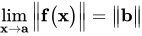
{\displaystyle \lim _{\mathbf {x} \to \mathbf {a} }{\Big \|}\mathbf {f} {\big (}\mathbf {x} {\big )}{\Big \|}={\big \|}\mathbf {b} {\big \|}}
Sabemos que a) e b) no teorema se verificam se
f
{\displaystyle f}
g
{\displaystyle g}
b
=
(
b
1
,
…
,
b
m
)
,
c
=
(
c
1
,
…
,
c
m
)
{\displaystyle \mathbf {b} ={\big (}b_{1},\ldots ,b_{m}{\big )},\mathbf {c} ={\big (}c_{1},\ldots ,c_{m}{\big )}}
a
)
f
(
x
)
=
[
f
1
(
x
)
,
…
,
f
m
(
x
)
]
,
g
(
x
)
=
[
g
1
(
x
)
,
…
,
g
m
(
x
)
]
lim
x
→
a
(
f
+
g
)
(
x
)
=
lim
x
→
a
[
(
f
1
+
g
1
)
(
x
)
,
…
,
(
f
m
+
g
m
)
(
x
)
]
=
[
lim
x
→
a
(
f
1
+
g
1
)
(
x
)
,
…
,
lim
x
→
a
(
f
m
+
g
m
)
(
x
)
]
=
[
lim
x
→
a
f
1
(
x
)
+
lim
x
→
a
g
1
(
x
)
,
…
,
lim
x
→
a
f
m
(
x
)
+
lim
x
→
a
g
m
(
x
)
]
=
(
b
1
+
c
1
,
…
,
b
m
+
c
m
)
=
(
b
1
,
…
,
b
m
)
+
(
c
1
,
…
,
c
m
)
=
b
+
c
{\displaystyle {\begin{array}{rl}a)&\mathbf {f} {\big (}\mathbf {x} )={\big [}f_{1}{\big (}\mathbf {x} {\big )},\ldots ,f_{m}{\big (}\mathbf {x} {\big )}{\big ]},\mathbf {g} {\big (}\mathbf {x} )={\Big [}g_{1}{\big (}\mathbf {x} {\big )},\ldots ,g_{m}{\big (}\mathbf {x} {\big )}{\Big ]}\\&\lim _{\mathbf {x} \to \mathbf {a} }{\big (}\mathbf {f} +\mathbf {g} {\big )}{\big (}\mathbf {x} {\big )}=\lim _{\mathbf {x} \to \mathbf {a} }{\Big [}{\big (}f_{1}+g_{1}{\big )}{\big (}\mathbf {x} {\big )},\ldots ,{\big (}f_{m}+g_{m}{\big )}{\big (}\mathbf {x} {\big )}{\Big ]}=\\&{\Big [}\lim _{\mathbf {x} \to \mathbf {a} }{\big (}f_{1}+g_{1}{\big )}{\big (}\mathbf {x} {\big )},\ldots ,\lim _{\mathbf {x} \to \mathbf {a} }{\big (}f_{m}+g_{m}{\big )}{\big (}\mathbf {x} {\big )}{\Big ]}=\\&{\Big [}\lim _{\mathbf {x} \to \mathbf {a} }f_{1}{\big (}\mathbf {x} {\big )}+\lim _{\mathbf {x} \to \mathbf {a} }g_{1}(\mathbf {x} {\big )},\ldots ,\lim _{\mathbf {x} \to \mathbf {a} }f_{m}{\big (}\mathbf {x} {\big )}+\lim _{\mathbf {x} \to \mathbf {a} }g_{m}{\big (}\mathbf {x} {\big )}{\Big ]}=\\&{\big (}b_{1}+c_{1},\ldots ,b_{m}+c_{m}{\big )}={\big (}b_{1},\ldots ,b_{m}{\big )}+{\big (}c_{1},\ldots ,c_{m}{\big )}=\mathbf {b} +\mathbf {c} \end{array}}}
b
)
lim
x
→
a
λ
f
(
x
)
=
lim
x
→
a
λ
[
f
1
(
x
)
,
…
,
f
m
(
x
)
]
=
lim
x
→
a
[
λ
f
1
(
x
)
,
…
,
λ
f
m
(
x
)
]
=
[
lim
x
→
a
λ
f
1
(
x
)
,
…
,
lim
x
→
a
λ
f
m
(
x
)
]
=
[
λ
lim
x
→
a
f
1
(
x
)
,
…
,
λ
lim
x
→
a
f
m
(
x
)
]
=
λ
[
lim
x
→
a
f
1
(
x
)
,
…
,
lim
x
→
a
f
m
(
x
)
]
=
λ
(
b
1
,
…
,
b
m
)
=
λ
b
{\displaystyle {\begin{array}{rl}b)&\lim _{\mathbf {x} \to \mathbf {a} }\lambda \mathbf {f} {\big (}\mathbf {x} {\big )}=\lim _{\mathbf {x} \to \mathbf {a} }\lambda {\Big [}f_{1}{\big (}\mathbf {x} {\big )},\ldots ,f_{m}{\big (}\mathbf {x} {\big )}{\Big ]}=\lim _{\mathbf {x} \to \mathbf {a} }{\Big [}\lambda f_{1}{\big (}\mathbf {x} {\big )},\ldots ,\lambda f_{m}{\big (}\mathbf {x} {\big )}{\Big ]}=\\&{\Big [}\lim _{\mathbf {x} \to \mathbf {a} }\lambda f_{1}{\big (}\mathbf {x} {\big )},\ldots ,\lim _{\mathbf {x} \to \mathbf {a} }\lambda f_{m}{\big (}\mathbf {x} {\big )}{\Big ]}={\Big [}\lambda \lim _{\mathbf {x} \to \mathbf {a} }f_{1}{\big (}\mathbf {x} {\big )},\ldots ,\lambda \lim _{\mathbf {x} \to \mathbf {a} }f_{m}{\big (}\mathbf {x} {\big )}{\Big ]}=\\&\lambda {\Big [}\lim _{\mathbf {x} \to \mathbf {a} }f_{1}{\big (}\mathbf {x} {\big )},\ldots ,\lim _{\mathbf {x} \to \mathbf {a} }f_{m}{\big (}\mathbf {x} {\big )}{\Big ]}=\lambda {\big (}b_{1},\ldots ,b_{m}{\big )}=\lambda \mathbf {b} \end{array}}}
c
)
(
f
⋅
g
)
(
x
)
−
b
⋅
c
=
[
f
(
x
)
−
b
]
⋅
[
g
(
x
)
−
c
]
+
b
⋅
[
g
(
x
)
−
c
]
+
c
⋅
[
f
(
x
)
−
b
]
{\displaystyle c)\quad {\big (}\mathbf {f} \cdot \mathbf {g} {\big )}{\big (}\mathbf {x} {\big )}-\mathbf {b} \cdot \mathbf {c} ={\Big [}\mathbf {f} {\big (}\mathbf {x} {\big )}-\mathbf {b} {\Big ]}\cdot {\Big [}\mathbf {g} {\big (}\mathbf {x} {\big )}-\mathbf {c} {\Big ]}+\mathbf {b} \cdot {\Big [}\mathbf {g} {\big (}\mathbf {x} {\big )}-\mathbf {c} {\Big ]}+\mathbf {c} \cdot {\Big [}\mathbf {f} {\big (}\mathbf {x} {\big )}-\mathbf {b} {\Big ]}}
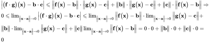
Aplicando a desigualdade triangular e a desigualdade de Cauchy-Schwarz temos
|
(
f
⋅
g
)
(
x
)
−
b
⋅
c
|
⩽
‖
f
(
x
)
−
b
‖
⋅
‖
g
(
x
)
−
c
‖
+
‖
b
‖
⋅
‖
g
(
x
)
−
c
‖
+
‖
c
‖
⋅
‖
f
(
x
)
−
b
‖
⇒
0
⩽
lim
‖
x
−
a
‖
→
0
|
(
f
⋅
g
)
(
x
)
−
b
⋅
c
|
⩽
lim
‖
x
−
a
‖
→
0
‖
f
(
x
)
−
b
‖
⋅
lim
‖
x
−
a
‖
→
0
‖
g
(
x
)
−
c
‖
+
‖
b
‖
⋅
lim
‖
x
−
a
‖
→
0
‖
g
(
x
)
−
c
‖
+
‖
c
‖
lim
‖
x
−
a
‖
→
0
‖
f
(
x
)
−
b
‖
=
0
⋅
0
+
‖
b
‖
⋅
0
+
‖
c
‖
⋅
0
=
0
{\displaystyle {\begin{array}{l}{\Big |}{\big (}\mathbf {f} \cdot \mathbf {g} {\big )}{\big (}\mathbf {x} {\big )}-\mathbf {b} \cdot \mathbf {c} {\Big |}\leqslant {\Big \|}\mathbf {f} {\big (}\mathbf {x} {\big )}-\mathbf {b} {\Big \|}\cdot {\Big \|}\mathbf {g} {\big (}\mathbf {x} {\big )}-\mathbf {c} {\Big \|}+{\big \|}\mathbf {b} {\big \|}\cdot {\Big \|}\mathbf {g} {\big (}\mathbf {x} {\big )}-\mathbf {c} {\Big \|}+{\big \|}\mathbf {c} {\big \|}\cdot {\Big \|}\mathbf {f} {\big (}\mathbf {x} {\big )}-\mathbf {b} {\Big \|}\Rightarrow \\0\leqslant \lim _{{\big \|}\mathbf {x} -\mathbf {a} {\big \|}\to 0}{\Big |}{\big (}\mathbf {f} \cdot \mathbf {g} {\big )}{\big (}\mathbf {x} {\big )}-\mathbf {b} \cdot \mathbf {c} {\Big |}\leqslant \lim _{{\big \|}\mathbf {x} -\mathbf {a} {\big \|}\to 0}{\Big \|}\mathbf {f} {\big (}\mathbf {x} {\big )}-\mathbf {b} {\Big \|}\cdot \lim _{{\big \|}\mathbf {x} -\mathbf {a} {\big \|}\to 0}{\Big \|}\mathbf {g} {\big (}\mathbf {x} {\big )}-\mathbf {c} {\Big \|}+\\{\big \|}\mathbf {b} {\big \|}\cdot \lim _{{\big \|}\mathbf {x} -\mathbf {a} {\big \|}\to 0}{\Big \|}\mathbf {g} {\big (}\mathbf {x} {\big )}-\mathbf {c} {\Big \|}+{\big \|}\mathbf {c} {\big \|}\lim _{{\big \|}\mathbf {x} -\mathbf {a} {\big \|}\to 0}{\Big \|}\mathbf {f} {\big (}\mathbf {x} {\big )}-\mathbf {b} {\Big \|}=0\cdot 0+{\big \|}\mathbf {b} {\big \|}\cdot 0+{\big \|}\mathbf {c} {\big \|}\cdot 0=\\0\end{array}}}
, como queríamos demonstrar.
d
)
g
(
x
)
=
f
(
x
)
,
c
=
b
⇒
lim
x
→
a
‖
f
(
x
)
‖
2
=
‖
b
‖
2
{\displaystyle d)\quad \mathbf {g} {\big (}\mathbf {x} {\big )}=\mathbf {f} {\big (}\mathbf {x} {\big )},\mathbf {c} =\mathbf {b} \Rightarrow \lim _{\mathbf {x} \to \mathbf {a} }{\Big \|}\mathbf {f} {\big (}\mathbf {x} {\big )}{\Big \|}^{2}={\big \|}\mathbf {b} {\big \|}^{2}}
Sejam
f
{\displaystyle \mathbf {f} }
g
{\displaystyle \mathbf {g} }
f
∘
g
{\displaystyle \mathbf {f} \circ \mathbf {g} }
a
{\displaystyle \mathbf {a} }
(
f
∘
g
)
(
x
)
=
f
[
g
(
x
)
]
{\displaystyle {\big (}\mathbf {f} \circ \mathbf {g} {\big )}{\big (}\mathbf {x} {\big )}=\mathbf {f} {\Big [}\mathbf {g} {\big (}\mathbf {x} {\big )}{\Big ]}}
g
{\displaystyle \mathbf {g} }
a
{\displaystyle \mathbf {a} }
f
{\displaystyle \mathbf {f} }
g
(
a
)
⇒
(
f
∘
g
)
{\displaystyle \mathbf {g} {\big (}\mathbf {a} {\big )}\Rightarrow {\big (}\mathbf {f} \circ \mathbf {g} {\big )}}
a
{\displaystyle \mathbf {a} }
Sejam
y
=
g
(
x
)
{\displaystyle \mathbf {y} =\mathbf {g} {\big (}\mathbf {x} {\big )}}
b
=
g
(
a
)
{\displaystyle \mathbf {b} =\mathbf {g} {\big (}\mathbf {a} {\big )}}
lim
‖
x
−
a
‖
→
0
‖
f
[
g
(
x
)
]
−
f
[
g
(
a
)
]
‖
=
lim
‖
y
−
b
‖
→
0
‖
f
(
y
)
−
f
(
b
)
‖
=
0
⇒
lim
x
→
a
f
[
g
(
x
)
]
=
f
[
g
(
a
)
]
{\displaystyle {\begin{array}{l}\lim _{{\big \|}\mathbf {x} -\mathbf {a} {\big \|}\to 0}{\Big \|}\mathbf {f} {\Big [}\mathbf {g} {\big (}\mathbf {x} {\big )}{\Big ]}-\mathbf {f} {\Big [}\mathbf {g} {\big (}\mathbf {a} {\big )}{\Big ]}{\Big \|}=\lim _{{\big \|}\mathbf {y} -\mathbf {b} {\big \|}\to 0}{\Big \|}\mathbf {f} {\big (}\mathbf {y} {\big )}-\mathbf {f} {\big (}\mathbf {b} {\big )}{\Big \|}=0\Rightarrow \\\lim _{\mathbf {x} \to \mathbf {a} }\mathbf {f} {\Big [}\mathbf {g} {\big (}\mathbf {x} {\big )}{\Big ]}=\mathbf {f} {\Big [}\mathbf {g} {\big (}\mathbf {a} {\big )}{\Big ]}\end{array}}}
como queríamos demostrar. Derivada de um campo escalar em relação a um vetor [ editar | editar código-fonte ] Seja
f
:
S
⊆
R
n
⟶
R
{\displaystyle f:S\subseteq \mathbb {R} ^{n}\longrightarrow \mathbb {R} }
x
{\displaystyle \mathbf {x} }
∈
S
,
{\displaystyle \in S,}
y
{\displaystyle \mathbf {y} }
R
n
{\displaystyle \mathbb {R} ^{n}}
f em
x
{\displaystyle \mathbf {x} }
y
{\displaystyle \mathbf {y} }
f
′
(
x
;
y
)
=
lim
h
→
0
f
(
x
+
h
y
)
−
f
(
x
)
h
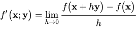
{\displaystyle f'{\big (}\mathbf {x} ;\mathbf {y} {\big )}=\lim _{h\to 0}{\cfrac {f{\big (}\mathbf {x} +h\mathbf {y} {\big )}-f{\big (}\mathbf {x} {\big )}}{h}}}
∂
f
∂
x
k
=
lim
h
→
0
f
(
x
1
,
…
,
x
k
+
h
,
…
,
x
n
)
−
f
(
x
1
,
…
,
x
k
,
…
,
x
n
)
h
{\displaystyle {\cfrac {\partial f}{\partial x_{k}}}=\lim _{h\to 0}{\cfrac {f{\big (}x_{1},\ldots ,x_{k}+h,\ldots ,x_{n}{\big )}-f{\big (}x_{1},\ldots ,x_{k},\ldots ,x_{n}{\big )}}{h}}}
Se derivamos a expressão anterior em relação a uma segunda variável,
x
j
{\displaystyle x_{j}}
∂
2
f
∂
x
j
∂
x
k
{\displaystyle {\cfrac {\partial ^{2}f}{\partial x_{j}\partial x_{k}}}}
∂
f
∂
x
k
{\displaystyle {\cfrac {\partial f}{\partial x_{k}}}}
x
k
{\displaystyle x_{k}}
x
j
,
∀
j
≠
k
{\displaystyle x_{j},\quad \forall j\neq k}
Dizemos que f é diferenciável em
a
⇔
{\displaystyle \mathbf {a} \Leftrightarrow }
∃
f
L
:
R
n
⟶
R
|
lim
‖
v
‖
→
0
f
(
a
+
v
)
=
f
(
a
)
+
f
L
(
v
)
{\displaystyle \exists f_{L}:\mathbb {R} ^{n}\longrightarrow \mathbb {R} {\Big |}\lim _{{\big \|}\mathbf {v} {\big \|}\to \mathbf {0} }f{\big (}\mathbf {a} +\mathbf {v} {\big )}=f{\big (}\mathbf {a} {\big )}+f_{L}{\big (}\mathbf {v} {\big )}}
f
L
{\displaystyle f_{L}}
aplicação linear , que definimos como a diferencial de f em a .A equação anterior é a fórmula de Taylor de primeira ordem para
f
(
a
+
v
)
{\displaystyle f{\big (}\mathbf {a} +\mathbf {v} {\big )}}
f
{\displaystyle f}
x
{\displaystyle \mathbf {x} }
f
L
(
y
)
⇒
{\displaystyle f_{L}{\big (}\mathbf {y} {\big )}\Rightarrow }
a)
∃
f
′
(
x
;
y
)
∀
y
∈
R
n
{\displaystyle \exists f'{\big (}\mathbf {x} ;\mathbf {y} {\big )}\quad \forall \mathbf {y} \in \mathbb {R} ^{n}}
b)
f
′
(
x
;
y
)
=
∑
k
=
1
n
y
k
∂
f
∂
x
k
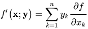
{\displaystyle f'{\big (}\mathbf {x} ;\mathbf {y} {\big )}=\sum _{k=1}^{n}y_{k}{\cfrac {\partial f}{\partial x_{k}}}}
a
)
v
=
h
y
,
h
∈
R
,
lim
‖
v
‖
→
0
f
(
x
+
v
)
=
lim
‖
v
‖
→
0
f
(
x
+
h
y
)
=
f
(
x
)
+
f
L
(
h
y
)
=
f
(
x
)
+
h
f
L
(
y
)
⇒
lim
h
→
0
f
(
x
+
h
y
)
−
f
(
x
)
h
=
f
′
(
x
;
y
)
=
f
L
(
y
)
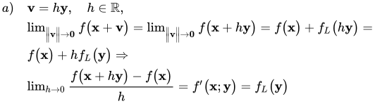
{\displaystyle {\begin{array}{rl}a)&\mathbf {v} =h\mathbf {y} ,\quad h\in \mathbb {R} ,\\&\lim _{{\big \|}\mathbf {v} {\big \|}\to \mathbf {0} }f{\big (}\mathbf {x} +\mathbf {v} {\big )}=\lim _{{\big \|}\mathbf {v} {\big \|}\to \mathbf {0} }f{\big (}\mathbf {x} +h\mathbf {y} {\big )}=f{\big (}\mathbf {x} {\big )}+f_{L}{\big (}h\mathbf {y} {\big )}=\\&f{\big (}\mathbf {x} {\big )}+hf_{L}{\big (}\mathbf {y} {\big )}\Rightarrow \\&\lim _{h\to 0}{\cfrac {f{\big (}\mathbf {x} +h\mathbf {y} {\big )}-f{\big (}\mathbf {x} {\big )}}{h}}=f'{\big (}\mathbf {x} ;\mathbf {y} {\big )}=f_{L}{\big (}\mathbf {y} {\big )}\end{array}}}
como queríamos demonstrar.
b
)
{\displaystyle b)}
y
{\displaystyle y}
{
e
1
,
…
,
e
n
}
,
f
L
(
y
)
=
f
L
(
∑
k
=
1
n
y
k
e
k
)
=
∑
k
=
1
n
y
k
f
L
(
e
k
)
=
∑
k
=
1
n
y
k
f
′
(
x
;
e
k
)
=
∑
k
=
1
n
y
k
∂
f
∂
x
k
{\displaystyle {\begin{array}{l}{\big \{}\mathbf {e} _{1},\ldots ,\mathbf {e} _{n}{\big \}},f_{L}{\big (}\mathbf {y} {\big )}=f_{L}{\big (}\sum _{k=1}^{n}y_{k}\mathbf {e} _{k}{\big )}=\sum _{k=1}^{n}y_{k}f_{L}{\big (}\mathbf {e} _{k}{\big )}=\sum _{k=1}^{n}y_{k}f'{\big (}\mathbf {x} ;\mathbf {e} _{k}{\big )}=\\\sum _{k=1}^{n}y_{k}{\cfrac {\partial f}{\partial x_{k}}}\end{array}}}
como queríamos demonstrar. Seja
f
:
S
⊂
R
n
⟶
R
{\displaystyle f:S\subset \mathbb {R} ^{n}\longrightarrow \mathbb {R} }
x
:
J
∈
R
⟶
S
{\displaystyle \mathbf {x} :J\in \mathbb {R} \longrightarrow S}
g
=
f
∘
x
{\displaystyle g=f\circ \mathbf {x} }
g
(
t
)
=
f
[
x
(
t
)
]
{\displaystyle g(t)=f{\Big [}\mathbf {x} {\big (}t{\big )}{\Big ]}}
g
′
(
t
)
=
∑
k
=
1
n
∂
f
∂
x
k
⋅
d
x
k
d
t
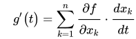
{\displaystyle \quad g'{\big (}t{\big )}=\sum _{k=1}^{n}{\cfrac {\partial f}{\partial x_{k}}}\cdot {\cfrac {dx_{k}}{dt}}}
Seja
f
:
S
⊆
R
n
⟶
R
m
{\displaystyle \mathbf {f} :S\subseteq \mathbb {R} ^{n}\longrightarrow \mathbb {R} ^{m}}
x
∈
S
{\displaystyle \mathbf {x} \in S}
y
{\displaystyle \mathbf {y} }
f
′
(
x
;
y
)
=
lim
h
→
0
f
(
x
+
h
y
)
−
f
(
x
)
h
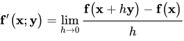
{\displaystyle \mathbf {f'} {\big (}\mathbf {x} ;\mathbf {y} {\big )}=\lim _{h\to 0}{\cfrac {\mathbf {f} {\big (}\mathbf {x} +h\mathbf {y} {\big )}-\mathbf {f} {\big (}\mathbf {x} {\big )}}{h}}}
Expressando
f
′
(
x
;
y
)
{\displaystyle \mathbf {f'} {\big (}\mathbf {x} ;\mathbf {y} {\big )}}
f
′
(
x
;
y
)
=
[
f
1
′
(
x
;
y
)
,
…
,
f
m
′
(
x
;
y
)
]
{\displaystyle \mathbf {f'} {\big (}\mathbf {x} ;\mathbf {y} {\big )}={\Big [}f'_{1}{\big (}\mathbf {x} ;\mathbf {y} {\big )},\ldots ,f'_{m}{\big (}\mathbf {x} ;\mathbf {y} {\big )}{\Big ]}}
Dizemos que
f
{\displaystyle \mathbf {f} }
⇔
∃
f
L
:
R
n
⟶
R
m
{\displaystyle \Leftrightarrow \exists \mathbf {f} _{L}:\mathbb {R} ^{n}\longrightarrow \mathbb {R} ^{m}}
aplicação linear que verifica:
lim
‖
v
‖
→
0
f
(
x
+
v
)
=
f
(
x
)
+
f
L
(
v
)
{\displaystyle \lim _{{\big \|}\mathbf {v} {\big \|}\to 0}\mathbf {f} {\big (}\mathbf {x} +\mathbf {v} {\big )}=\mathbf {f} {\big (}\mathbf {x} {\big )}+\mathbf {f} _{L}{\big (}\mathbf {v} {\big )}}
Esta é a fórmula de Taylor de primeira ordem para
f
.
f
L
(
v
)
=
f
′
(
x
;
v
)
{\displaystyle \mathbf {f} .\quad \mathbf {f} _{L}{\big (}\mathbf {v} {\big )}=\mathbf {f} '{\big (}\mathbf {x} ;\mathbf {v} {\big )}}
A matriz de
f
′
{\displaystyle \mathbf {f} '}
matriz jacobiana .
Se um campo vetorial
f
{\displaystyle \mathbf {f} }
diferenciável em
x
⇒
{\displaystyle \mathbf {x} \Rightarrow }
contínuo em
x
{\displaystyle \mathbf {x} }
Se deduze facilmente da fórmula de Taylor de primeira ordem já vista. Regra da cadeia para diferenciais de campos vetoriais [ editar | editar código-fonte ] Seja
h
(
x
)
=
(
f
∘
g
)
(
x
)
{\displaystyle \mathbf {h} {\big (}\mathbf {x} {\big )}={\big (}\mathbf {f} \circ \mathbf {g} {\big )}{\big (}\mathbf {x} {\big )}}
x
{\displaystyle \mathbf {x} }
h
′
(
x
)
{\displaystyle \mathbf {h} '{\big (}\mathbf {x} {\big )}}
h
′
(
x
)
=
f
′
[
g
(
x
)
]
∘
g
′
(
x
)
{\displaystyle \mathbf {h} '{\big (}\mathbf {x} {\big )}=\mathbf {f} '{\Big [}\mathbf {g} {\big (}\mathbf {x} {\big )}{\Big ]}\circ \mathbf {g} '{\big (}\mathbf {x} {\big )}}
Condição suficiente para a igualdade das derivadas parciais mistas [ editar | editar código-fonte ]
∂
2
f
∂
x
i
∂
x
j
=
∂
2
f
∂
x
j
∂
x
i
∀
i
≠
j
⇔
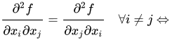
{\displaystyle {\cfrac {\partial ^{2}f}{\partial x_{i}\partial x_{j}}}={\cfrac {\partial ^{2}f}{\partial x_{j}\partial x_{i}}}\quad \forall i\neq j\Leftrightarrow }
x
{\displaystyle \mathbf {x} }
Um campo escalar tem um máximo em
x
=
a
⇔
{\displaystyle \mathbf {x} =\mathbf {a} \Leftrightarrow }
n -esfera
B
(
a
)
|
∀
x
∈
B
(
a
)
f
(
x
)
⩽
f
(
a
)
{\displaystyle B{\big (}\mathbf {a} {\big )}{\Big |}\forall \mathbf {x} \in B{\big (}\mathbf {a} {\big )}\quad f{\big (}\mathbf {x} {\big )}\leqslant f{\big (}\mathbf {a} {\big )}}
Um campo escalar tem um mínimo em
x
=
a
⇔
{\displaystyle \mathbf {x} =\mathbf {a} \Leftrightarrow }
n -esfera
B
(
a
)
|
∀
x
∈
B
(
a
)
f
(
x
)
⩾
f
(
a
)
{\displaystyle B{\big (}\mathbf {a} {\big )}{\Big |}\forall \mathbf {x} \in B{\big (}\mathbf {a} {\big )}\quad f{\big (}\mathbf {x} {\big )}\geqslant f{\big (}\mathbf {a} {\big )}}
Um campo escalar tem um ponto de sela
⇔
{\displaystyle \Leftrightarrow }
∀
B
(
a
)
∃
x
|
f
(
x
)
⩽
f
(
a
)
∧
∃
x
|
f
(
x
)
⩾
f
(
a
)
{\displaystyle \forall B{\big (}\mathbf {a} {\big )}\quad \exists \mathbf {x} {\big |}f{\big (}\mathbf {x} {\big )}\leqslant f{\big (}\mathbf {a} {\big )}\land \exists \mathbf {x} {\big |}f{\big (}\mathbf {x} {\big )}\geqslant f{\big (}\mathbf {a} {\big )}}
Função com um ponto de sela . Para saber se é um dos casos anteriores:
Obtemos
x
|
∂
f
∂
x
k
=
0
∀
k
|
1
⩽
k
⩽
n
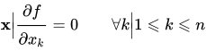
{\displaystyle \mathbf {x} {\Big |}{\cfrac {\partial f}{\partial x_{k}}}=0\qquad \forall k{\Big |}1\leqslant k\leqslant n}
Obtemos a matriz hessiana de f . Seja esta
F
(
x
)
{\displaystyle \mathbf {F} {\big (}\mathbf {x} {\big )}}
F
(
x
)
{\displaystyle \mathbf {F} {\big (}\mathbf {x} {\big )}}
definida positiva
⇒
f
{\displaystyle \Rightarrow f}
mínimo local (mínimo relativo ) em
x
{\displaystyle \mathbf {x} }
F
(
x
)
{\displaystyle \mathbf {F} {\big (}\mathbf {x} {\big )}}
definida negativa
⇒
f
{\displaystyle \Rightarrow f}
máximo local (máximo relativo ) em
x
{\displaystyle \mathbf {x} }
F
(
x
)
{\displaystyle \mathbf {F} {\big (}\mathbf {x} {\big )}}
indefinida
⇒
f
{\displaystyle \Rightarrow f}
ponto de sela em
x
{\displaystyle \mathbf {x} }
No exposto anteriormente, supomos que
∂
2
f
∂
x
i
∂
x
j
{\displaystyle {\cfrac {\partial ^{2}f}{\partial x_{i}\partial x_{j}}}}
∀
i
,
j
|
1
⩽
i
⩽
n
,
1
⩽
j
⩽
n
{\displaystyle \forall i,j{\big |}1\leqslant i\leqslant n,1\leqslant j\leqslant n}
Referências

















![{\displaystyle \lim _{\mathbf {x} \to \mathbf {a} }{\big [}\mathbf {f} +\mathbf {g} {\big ]}{\big (}\mathbf {x} {\big )}=\mathbf {b} +\mathbf {c} }](https://wikimedia.org/api/rest_v1/media/math/render/svg/97e7d295bd1d5497f0c98c4d16c52d2720d749d0)







![{\displaystyle {\begin{array}{rl}a)&\mathbf {f} {\big (}\mathbf {x} )={\big [}f_{1}{\big (}\mathbf {x} {\big )},\ldots ,f_{m}{\big (}\mathbf {x} {\big )}{\big ]},\mathbf {g} {\big (}\mathbf {x} )={\Big [}g_{1}{\big (}\mathbf {x} {\big )},\ldots ,g_{m}{\big (}\mathbf {x} {\big )}{\Big ]}\\&\lim _{\mathbf {x} \to \mathbf {a} }{\big (}\mathbf {f} +\mathbf {g} {\big )}{\big (}\mathbf {x} {\big )}=\lim _{\mathbf {x} \to \mathbf {a} }{\Big [}{\big (}f_{1}+g_{1}{\big )}{\big (}\mathbf {x} {\big )},\ldots ,{\big (}f_{m}+g_{m}{\big )}{\big (}\mathbf {x} {\big )}{\Big ]}=\\&{\Big [}\lim _{\mathbf {x} \to \mathbf {a} }{\big (}f_{1}+g_{1}{\big )}{\big (}\mathbf {x} {\big )},\ldots ,\lim _{\mathbf {x} \to \mathbf {a} }{\big (}f_{m}+g_{m}{\big )}{\big (}\mathbf {x} {\big )}{\Big ]}=\\&{\Big [}\lim _{\mathbf {x} \to \mathbf {a} }f_{1}{\big (}\mathbf {x} {\big )}+\lim _{\mathbf {x} \to \mathbf {a} }g_{1}(\mathbf {x} {\big )},\ldots ,\lim _{\mathbf {x} \to \mathbf {a} }f_{m}{\big (}\mathbf {x} {\big )}+\lim _{\mathbf {x} \to \mathbf {a} }g_{m}{\big (}\mathbf {x} {\big )}{\Big ]}=\\&{\big (}b_{1}+c_{1},\ldots ,b_{m}+c_{m}{\big )}={\big (}b_{1},\ldots ,b_{m}{\big )}+{\big (}c_{1},\ldots ,c_{m}{\big )}=\mathbf {b} +\mathbf {c} \end{array}}}](https://wikimedia.org/api/rest_v1/media/math/render/svg/95faf263a1baf0db2c17757d92d4652b8000a3c0)
![{\displaystyle {\begin{array}{rl}b)&\lim _{\mathbf {x} \to \mathbf {a} }\lambda \mathbf {f} {\big (}\mathbf {x} {\big )}=\lim _{\mathbf {x} \to \mathbf {a} }\lambda {\Big [}f_{1}{\big (}\mathbf {x} {\big )},\ldots ,f_{m}{\big (}\mathbf {x} {\big )}{\Big ]}=\lim _{\mathbf {x} \to \mathbf {a} }{\Big [}\lambda f_{1}{\big (}\mathbf {x} {\big )},\ldots ,\lambda f_{m}{\big (}\mathbf {x} {\big )}{\Big ]}=\\&{\Big [}\lim _{\mathbf {x} \to \mathbf {a} }\lambda f_{1}{\big (}\mathbf {x} {\big )},\ldots ,\lim _{\mathbf {x} \to \mathbf {a} }\lambda f_{m}{\big (}\mathbf {x} {\big )}{\Big ]}={\Big [}\lambda \lim _{\mathbf {x} \to \mathbf {a} }f_{1}{\big (}\mathbf {x} {\big )},\ldots ,\lambda \lim _{\mathbf {x} \to \mathbf {a} }f_{m}{\big (}\mathbf {x} {\big )}{\Big ]}=\\&\lambda {\Big [}\lim _{\mathbf {x} \to \mathbf {a} }f_{1}{\big (}\mathbf {x} {\big )},\ldots ,\lim _{\mathbf {x} \to \mathbf {a} }f_{m}{\big (}\mathbf {x} {\big )}{\Big ]}=\lambda {\big (}b_{1},\ldots ,b_{m}{\big )}=\lambda \mathbf {b} \end{array}}}](https://wikimedia.org/api/rest_v1/media/math/render/svg/10fef6b37ec01f2a38f73284854a3e4d6b80462c)
![{\displaystyle c)\quad {\big (}\mathbf {f} \cdot \mathbf {g} {\big )}{\big (}\mathbf {x} {\big )}-\mathbf {b} \cdot \mathbf {c} ={\Big [}\mathbf {f} {\big (}\mathbf {x} {\big )}-\mathbf {b} {\Big ]}\cdot {\Big [}\mathbf {g} {\big (}\mathbf {x} {\big )}-\mathbf {c} {\Big ]}+\mathbf {b} \cdot {\Big [}\mathbf {g} {\big (}\mathbf {x} {\big )}-\mathbf {c} {\Big ]}+\mathbf {c} \cdot {\Big [}\mathbf {f} {\big (}\mathbf {x} {\big )}-\mathbf {b} {\Big ]}}](https://wikimedia.org/api/rest_v1/media/math/render/svg/66af9fd2140f9780543400554816ae1043fbe68f)



![{\displaystyle {\big (}\mathbf {f} \circ \mathbf {g} {\big )}{\big (}\mathbf {x} {\big )}=\mathbf {f} {\Big [}\mathbf {g} {\big (}\mathbf {x} {\big )}{\Big ]}}](https://wikimedia.org/api/rest_v1/media/math/render/svg/6e050e088fa87cd14516180f245242f9c90b4d73)


![{\displaystyle {\begin{array}{l}\lim _{{\big \|}\mathbf {x} -\mathbf {a} {\big \|}\to 0}{\Big \|}\mathbf {f} {\Big [}\mathbf {g} {\big (}\mathbf {x} {\big )}{\Big ]}-\mathbf {f} {\Big [}\mathbf {g} {\big (}\mathbf {a} {\big )}{\Big ]}{\Big \|}=\lim _{{\big \|}\mathbf {y} -\mathbf {b} {\big \|}\to 0}{\Big \|}\mathbf {f} {\big (}\mathbf {y} {\big )}-\mathbf {f} {\big (}\mathbf {b} {\big )}{\Big \|}=0\Rightarrow \\\lim _{\mathbf {x} \to \mathbf {a} }\mathbf {f} {\Big [}\mathbf {g} {\big (}\mathbf {x} {\big )}{\Big ]}=\mathbf {f} {\Big [}\mathbf {g} {\big (}\mathbf {a} {\big )}{\Big ]}\end{array}}}](https://wikimedia.org/api/rest_v1/media/math/render/svg/9e0972f84a181ff7e0e1de0688a2b517a3becc0b)

















![{\displaystyle g(t)=f{\Big [}\mathbf {x} {\big (}t{\big )}{\Big ]}}](https://wikimedia.org/api/rest_v1/media/math/render/svg/c24d0a6ebe6f93545e22280032f94396d0320cf9)



![{\displaystyle \mathbf {f'} {\big (}\mathbf {x} ;\mathbf {y} {\big )}={\Big [}f'_{1}{\big (}\mathbf {x} ;\mathbf {y} {\big )},\ldots ,f'_{m}{\big (}\mathbf {x} ;\mathbf {y} {\big )}{\Big ]}}](https://wikimedia.org/api/rest_v1/media/math/render/svg/b886201a23ee2c88781d76fe6abf5585db77bc24)







![{\displaystyle \mathbf {h} '{\big (}\mathbf {x} {\big )}=\mathbf {f} '{\Big [}\mathbf {g} {\big (}\mathbf {x} {\big )}{\Big ]}\circ \mathbf {g} '{\big (}\mathbf {x} {\big )}}](https://wikimedia.org/api/rest_v1/media/math/render/svg/7ee4c8d71f25c0b0392d15f41ec44fa1b485ee56)