
Usuário(a):Wcris~ptwiki/qft
Predefinição:Quantum field theory Quantum field theory or QFT[1] provides a theoretical framework for constructing quantum mechanical models of systems classically described by fields or of many-body systems. It is widely used in particle physics and condensed matter physics. Most theories in modern particle physics, including the Standard Model of elementary particles and their interactions, are formulated as relativistic quantum field theories. In condensed matter physics, quantum field theories are used in many circumstances, especially those where the number of particles is allowed to fluctuate—for example, in the BCS theory of superconductivity.
In quantum field theory (QFT) the forces between particles are mediated by other particles. The electromagnetic force between two electrons is caused by an exchange of photons. Intermediate vector bosons mediate the weak force and gluons mediate the strong force. There is currently no complete quantum theory of the remaining fundamental force, gravity, but many of the proposed theories postulate the existence of a graviton particle which mediates it. These force-carrying particles are virtual particles and, by definition, cannot be detected while carrying the force, because such detection will imply that the force is not being carried.
In QFT photons are not thought of as 'little billiard balls', they are considered to be field quanta - necessarily chunked ripples in a field that 'look like' particles. Fermions, like the electron, can also be described as ripples in a field, where each kind of fermion has its own field. In summary, the classical visualisation of "everything is particles and fields", in quantum field theory, resolves into "everything is particles", which then resolves into "everything is fields". In the end, particles are regarded as excited states of a field (field quanta).
History[editar | editar código-fonte]
Quantum field theory originated in the 1920s from the problem of creating a quantum mechanical theory of the electromagnetic field. In 1926, Max Born, Pascual Jordan, and Werner Heisenberg constructed such a theory by expressing the field's internal degrees of freedom as an infinite set of harmonic oscillators and by employing the usual procedure for quantizing those oscillators (canonical quantization). This theory assumed that no electric charges or currents were present and today would be called a free field theory. The first reasonably complete theory of quantum electrodynamics, which included both the electromagnetic field and electrically charged matter (specifically, electrons) as quantum mechanical objects, was created by Paul Dirac in 1927. This quantum field theory could be used to model important processes such as the emission of a photon by an electron dropping into a quantum state of lower energy, a process in which the number of particles changes — one atom in the initial state becomes an atom plus a photon in the final state. It is now understood that the ability to describe such processes is one of the most important features of quantum field theory.
It was evident from the beginning that a proper quantum treatment of the electromagnetic field had to somehow incorporate Einstein's relativity theory, which had after all grown out of the study of classical electromagnetism. This need to put together relativity and quantum mechanics was the second major motivation in the development of quantum field theory. Pascual Jordan and Wolfgang Pauli showed in 1928 that quantum fields could be made to behave in the way predicted by special relativity during coordinate transformations (specifically, they showed that the field commutators were Lorentz invariant), and in 1933 Niels Bohr and Leon Rosenfeld showed that this result could be interpreted as a limitation on the ability to measure fields at space-like separations, exactly as required by relativity. A further boost for quantum field theory came with the discovery of the Dirac equation, a single-particle equation obeying both relativity and quantum mechanics, when it was shown that several of its undesirable properties (such as negative-energy states) could be eliminated by reformulating the Dirac equation as a quantum field theory. This work was performed by Wendell Furry, Robert Oppenheimer, Vladimir Fock, and others.
The third thread in the development of quantum field theory was the need to handle the statistics of many-particle systems consistently and with ease. In 1927, Jordan tried to extend the canonical quantization of fields to the many-body wavefunctions of identical particles, a procedure that is sometimes called second quantization. In 1928, Jordan and Eugene Wigner found that the quantum field describing electrons, or other fermions, had to be expanded using anti-commuting creation and annihilation operators due to the Pauli exclusion principle. This thread of development was incorporated into many-body theory, and strongly influenced condensed matter physics and nuclear physics.
Despite its early successes, quantum field theory was plagued by several serious theoretical difficulties. Many seemingly-innocuous physical quantities, such as the energy shift of electron states due to the presence of the electromagnetic field, gave infinity — a nonsensical result — when computed using quantum field theory. This "divergence problem" was solved during the 1940s by Bethe, Tomonaga, Schwinger, Feynman, and Dyson, through the procedure known as renormalization. This phase of development culminated with the construction of the modern theory of quantum electrodynamics (QED). Beginning in the 1950s with the work of Yang and Mills, QED was generalized to a class of quantum field theories known as gauge theories. The 1960s and 1970s saw the formulation of a gauge theory now known as the Standard Model of particle physics, which describes all known elementary particles and the interactions between them. The weak interaction part of the standard model was formulated by Sheldon Glashow, with the Higgs mechanism added by Steven Weinberg and Abdus Salam. The theory was shown to be renormalizable and hence consistent by Gerardus 't Hooft and Martinus Veltman.
Also during the 1970s, parallel developments in the study of phase transitions in condensed matter physics led Leo Kadanoff, Michael Fisher and Kenneth Wilson (extending work of Ernst Stueckelberg, Andre Peterman, Murray Gell-Mann and Francis Low) to a set of ideas and methods known as the renormalization group. By providing a better physical understanding of the renormalization procedure invented in the 1940s, the renormalization group sparked what has been called the "grand synthesis" of theoretical physics, uniting the quantum field theoretical techniques used in particle physics and condensed matter physics into a single theoretical framework.
The study of quantum field theory is alive and flourishing, as are applications of this method to many physical problems. It remains one of the most vital areas of theoretical physics today, providing a common language to many branches of physics.
Principles of quantum field theory[editar | editar código-fonte]
Classical fields and quantum fields[editar | editar código-fonte]
Quantum mechanics, in its most general formulation, is a theory of abstract operators (observables) acting on an abstract state space (Hilbert space), where the observables represent physically-observable quantities and the state space represents the possible states of the system under study. Furthermore, each observable corresponds, in a technical sense, to the classical idea of a degree of freedom. For instance, the fundamental observables associated with the motion of a single quantum mechanical particle are the position and momentum operators and . Ordinary quantum mechanics deals with systems such as this, which possess a small set of degrees of freedom.


(It is important to note, at this point, that this article does not use the word "particle" in the context of wave–particle duality. In quantum field theory, "particle" is a generic term for any discrete quantum mechanical entity, such as an electron, which can behave like classical particles or classical waves under different experimental conditions.)
A quantum field is a quantum mechanical system containing a large, and possibly infinite, number of degrees of freedom. This is not as exotic a situation as one might think. A classical field contains a set of degrees of freedom at each point of space; for instance, the classical electromagnetic field defines two vectors — the electric field and the magnetic field — that can in principle take on distinct values for each position . When the field as a whole is considered as a quantum mechanical system, its observables form an infinite (in fact uncountable) set, because is continuous.

Furthermore, the degrees of freedom in a quantum field are arranged in "repeated" sets. For example, the degrees of freedom in an electromagnetic field can be grouped according to the position , with exactly two vectors for each . Note that is an ordinary number that "indexes" the observables; it is not to be confused with the position operator encountered in ordinary quantum mechanics, which is an observable. (Thus, ordinary quantum mechanics is sometimes referred to as "zero-dimensional quantum field theory", because it contains only a single set of observables.) It is also important to note that there is nothing special about because, as it turns out, there is generally more than one way of indexing the degrees of freedom in the field.
In the following sections, we will show how these ideas can be used to construct a quantum mechanical theory with the desired properties. We will begin by discussing single-particle quantum mechanics and the associated theory of many-particle quantum mechanics. Then, by finding a way to index the degrees of freedom in the many-particle problem, we will construct a quantum field and study its implications.
Single-particle and many-particle quantum mechanics[editar | editar código-fonte]
In ordinary quantum mechanics, the time-dependent Schrödinger equation describing the time evolution of the quantum state of a single non-relativistic particle is
![{\displaystyle \left[{\frac {|\mathbf {p} |^{2}}{2m}}+V(\mathbf {r} )\right]|\psi (t)\rangle =i\hbar {\frac {\partial }{\partial t}}|\psi (t)\rangle ,}](https://wikimedia.org/api/rest_v1/media/math/render/svg/5925118104b7a542f949ba5c36a5e051b474fab4)
where is the particle's mass, is the applied potential, and denotes the quantum state (we are using bra-ket notation).


We wish to consider how this problem generalizes to particles. There are two motivations for studying the many-particle problem. The first is a straightforward need in condensed matter physics, where typically the number of particles is on the order of Avogadro's number (6.0221415 x 10²³). The second motivation for the many-particle problem arises from particle physics and the desire to incorporate the effects of special relativity. If one attempts to include the relativistic rest energy into the above equation, the result is either the Klein-Gordon equation or the Dirac equation. However, these equations have many unsatisfactory qualities; for instance, they possess energy eigenvalues which extend to –∞, so that there seems to be no easy definition of a ground state. It turns out that such inconsistencies arise from neglecting the possibility of dynamically creating or destroying particles, which is a crucial aspect of relativity. Einstein's famous mass-energy relation predicts that sufficiently massive particles can decay into several lighter particles, and sufficiently energetic particles can combine to form massive particles. For example, an electron and a positron can annihilate each other to create photons. Thus, a consistent relativistic quantum theory must be formulated as a many-particle theory.

Furthermore, we will assume that the particles are indistinguishable. As described in the article on identical particles, this implies that the state of the entire system must be either symmetric (bosons) or antisymmetric (fermions) when the coordinates of its constituent particles are exchanged. These multi-particle states are rather complicated to write. For example, the general quantum state of a system of bosons is written as

where are the single-particle states, is the number of particles occupying state , and the sum is taken over all possible permutations acting on elements. In general, this is a sum of ( factorial) distinct terms, which quickly becomes unmanageable as increases. The way to simplify this problem is to turn it into a quantum field theory.


Second quantization[editar | editar código-fonte]
In this section, we will describe a method for constructing a quantum field theory called second quantization. This basically involves choosing a way to index the quantum mechanical degrees of freedom in the space of multiple identical-particle states. It is based on the Hamiltonian formulation of quantum mechanics; several other approaches exist, such as the Feynman path integral[2], which uses a Lagrangian formulation. For an overview, see the article on quantization.
Second quantization of bosons[editar | editar código-fonte]
For simplicity, we will first discuss second quantization for bosons, which form perfectly symmetric quantum states. Let us denote the mutually orthogonal single-particle states by and so on. For example, the 3-particle state with one particle in state and two in state is


![{\displaystyle {\frac {1}{\sqrt {3}}}\left[|\phi _{1}\rangle |\phi _{2}\rangle |\phi _{2}\rangle +|\phi _{2}\rangle |\phi _{1}\rangle |\phi _{2}\rangle +|\phi _{2}\rangle |\phi _{2}\rangle |\phi _{1}\rangle \right].}](https://wikimedia.org/api/rest_v1/media/math/render/svg/0c02fe5c2f1b38d579baca0380d95701289784be)
The first step in second quantization is to express such quantum states in terms of occupation numbers, by listing the number of particles occupying each of the single-particle states etc. This is simply another way of labelling the states. For instance, the above 3-particle state is denoted as


The next step is to expand the -particle state space to include the state spaces for all possible values of . This extended state space, known as a Fock space, is composed of the state space of a system with no particles (the so-called vacuum state), plus the state space of a 1-particle system, plus the state space of a 2-particle system, and so forth. It is easy to see that there is a one-to-one correspondence between the occupation number representation and valid boson states in the Fock space.
At this point, the quantum mechanical system has become a quantum field in the sense we described above. The field's elementary degrees of freedom are the occupation numbers, and each occupation number is indexed by a number , indicating which of the single-particle states it refers to.


The properties of this quantum field can be explored by defining creation and annihilation operators, which add and subtract particles. They are analogous to "ladder operators" in the quantum harmonic oscillator problem, which added and subtracted energy quanta. However, these operators literally create and annihilate particles of a given quantum state. The bosonic annihilation operator and creation operator have the following effects:


It can be shown that these are operators in the usual quantum mechanical sense, i.e. linear operators acting on the Fock space. Furthermore, they are indeed Hermitian conjugates, which justifies the way we have written them. They can be shown to obey the commutation relation
![{\displaystyle \left[a_{i},a_{j}\right]=0\quad ,\quad \left[a_{i}^{\dagger },a_{j}^{\dagger }\right]=0\quad ,\quad \left[a_{i},a_{j}^{\dagger }\right]=\delta _{ij},}](https://wikimedia.org/api/rest_v1/media/math/render/svg/5e9b906839a0d891c27f69c1d2a9a1f0d7bfda8f)
where stands for the Kronecker delta. These are precisely the relations obeyed by the ladder operators for an infinite set of independent quantum harmonic oscillators, one for each single-particle state. Adding or removing bosons from each state is therefore analogous to exciting or de-exciting a quantum of energy in a harmonic oscillator.

The Hamiltonian of the quantum field (which, through the Schrödinger equation, determines its dynamics) can be written in terms of creation and annihilation operators. For instance, the Hamiltonian of a field of free (non-interacting) bosons is

where is the energy of the -th single-particle energy eigenstate. Note that


Second quantization of fermions[editar | editar código-fonte]
It turns out that a different definition of creation and annihilation must be used for describing fermions. According to the Pauli exclusion principle, fermions cannot share quantum states, so their occupation numbers can only take on the value 0 or 1. The fermionic annihilation operators and creation operators are defined by


These obey an anticommutation relation:

One may notice from this that applying a fermionic creation operator twice gives zero, so it is impossible for the particles to share single-particle states, in accordance with the exclusion principle.
Field operators[editar | editar código-fonte]
We have previously mentioned that there can be more than one way of indexing the degrees of freedom in a quantum field. Second quantization indexes the field by enumerating the single-particle quantum states. However, as we have discussed, it is more natural to think about a "field", such as the electromagnetic field, as a set of degrees of freedom indexed by position.
To this end, we can define field operators that create or destroy a particle at a particular point in space. In particle physics, these operators turn out to be more convenient to work with, because they make it easier to formulate theories that satisfy the demands of relativity.
Single-particle states are usually enumerated in terms of their momenta (as in the particle in a box problem.) We can construct field operators by applying the Fourier transform to the creation and annihilation operators for these states. For example, the bosonic field annihilation operator is


The bosonic field operators obey the commutation relation
![{\displaystyle \left[\phi (\mathbf {r} ),\phi (\mathbf {r'} )\right]=0\quad ,\quad \left[\phi ^{\dagger }(\mathbf {r} ),\phi ^{\dagger }(\mathbf {r'} )\right]=0\quad ,\quad \left[\phi (\mathbf {r} ),\phi ^{\dagger }(\mathbf {r'} )\right]=\delta ^{3}(\mathbf {r} -\mathbf {r'} )}](https://wikimedia.org/api/rest_v1/media/math/render/svg/797eef6c468525e66ae8630aa8f35f65741b84b9)
where stands for the Dirac delta function. As before, the fermionic relations are the same, with the commutators replaced by anticommutators.

It should be emphasized that the field operator is not the same thing as a single-particle wavefunction. The former is an operator acting on the Fock space, and the latter is just a scalar field. However, they are closely related, and are indeed commonly denoted with the same symbol. If we have a Hamiltonian with a space representation, say

where the indices and run over all particles, then the field theory Hamiltonian is


This looks remarkably like an expression for the expectation value of the energy, with playing the role of the wavefunction. This relationship between the field operators and wavefunctions makes it very easy to formulate field theories starting from space-projected Hamiltonians.

Implications of quantum field theory[editar | editar código-fonte]
Unification of fields and particles[editar | editar código-fonte]
The "second quantization" procedure that we have outlined in the previous section takes a set of single-particle quantum states as a starting point. Sometimes, it is impossible to define such single-particle states, and one must proceed directly to quantum field theory. For example, a quantum theory of the electromagnetic field must be a quantum field theory, because it is impossible (for various reasons) to define a wavefunction for a single photon. In such situations, the quantum field theory can be constructed by examining the mechanical properties of the classical field and guessing the corresponding quantum theory. The quantum field theories obtained in this way have the same properties as those obtained using second quantization, such as well-defined creation and annihilation operators obeying commutation or anticommutation relations.
Quantum field theory thus provides a unified framework for describing "field-like" objects (such as the electromagnetic field, whose excitations are photons) and "particle-like" objects (such as electrons, which are treated as excitations of an underlying electron field).
Physical meaning of particle indistinguishability[editar | editar código-fonte]
The second quantization procedure relies crucially on the particles being identical. We would not have been able to construct a quantum field theory from a distinguishable many-particle system, because there would have been no way of separating and indexing the degrees of freedom.
Many physicists prefer to take the converse interpretation, which is that quantum field theory explains what identical particles are. In ordinary quantum mechanics, there is not much theoretical motivation for using symmetric (bosonic) or antisymmetric (fermionic) states, and the need for such states is simply regarded as an empirical fact. From the point of view of quantum field theory, particles are identical if and only if they are excitations of the same underlying quantum field. Thus, the question "why are all electrons identical?" arises from mistakenly regarding individual electrons as fundamental objects, when in fact it is only the electron field that is fundamental.
Particle conservation and non-conservation[editar | editar código-fonte]
During second quantization, we started with a Hamiltonian and state space describing a fixed number of particles (), and ended with a Hamiltonian and state space for an arbitrary number of particles. Of course, in many common situations is an important and perfectly well-defined quantity, e.g. if we are describing a gas of atoms sealed in a box. From the point of view of quantum field theory, such situations are described by quantum states that are eigenstates of the number operator , which measures the total number of particles present. As with any quantum mechanical observable, is conserved if it commutes with the Hamiltonian. In that case, the quantum state is trapped in the -particle subspace of the total Fock space, and the situation could equally well be described by ordinary -particle quantum mechanics.

For example, we can see that the free-boson Hamiltonian described above conserves particle number. Whenever the Hamiltonian operates on a state, each particle destroyed by an annihilation operator is immediately put back by the creation operator .


On the other hand, it is possible, and indeed common, to encounter quantum states that are not eigenstates of , which do not have well-defined particle numbers. Such states are difficult or impossible to handle using ordinary quantum mechanics, but they can be easily described in quantum field theory as quantum superpositions of states having different values of . For example, suppose we have a bosonic field whose particles can be created or destroyed by interactions with a fermionic field. The Hamiltonian of the combined system would be given by the Hamiltonians of the free boson and free fermion fields, plus a "potential energy" term such as
- ,

where and denotes the bosonic creation and annihilation operators, and denotes the fermionic creation and annihilation operators, and is a parameter that describes the strength of the interaction. This "interaction term" describes processes in which a fermion in state either absorbs or emits a boson, thereby being kicked into a different eigenstate . (In fact, this type of Hamiltonian is used to describe interaction between conduction electrons and phonons in metals. The interaction between electrons and photons is treated in a similar way, but is a little more complicated because the role of spin must be taken into account.) One thing to notice here is that even if we start out with a fixed number of bosons, we will typically end up with a superposition of states with different numbers of bosons at later times. The number of fermions, however, is conserved in this case.


In condensed matter physics, states with ill-defined particle numbers are particularly important for describing the various superfluids. Many of the defining characteristics of a superfluid arise from the notion that its quantum state is a superposition of states with different particle numbers.
Axiomatic approaches[editar | editar código-fonte]
The preceding description of quantum field theory follows the spirit in which most physicists approach the subject. However, it is not mathematically rigorous. Over the past several decades, there have been many attempts to put quantum field theory on a firm mathematical footing by formulating a set of axioms for it. These attempts fall into two broad classes.
The first class of axioms, first proposed during the 1950s, include the Wightman, Osterwalder-Schrader, and Haag-Kastler systems. They attempted to formalize the physicists' notion of an "operator-valued field" within the context of functional analysis, and enjoyed limited success. It was possible to prove that any quantum field theory satisfying these axioms satisfied certain general theorems, such as the spin-statistics theorem and the CPT theorem. Unfortunately, it proved extraordinarily difficult to show that any realistic field theory, including the Standard Model, satisfied these axioms. Most of the theories that could be treated with these analytic axioms were physically trivial, being restricted to low-dimensions and lacking interesting dynamics. The construction of theories satisfying one of these sets of axioms falls in the field of constructive quantum field theory. Important work was done in this area in the 1970s by Segal, Glimm, Jaffe and others.
During the 1980s, a second set of axioms based on geometric ideas was proposed. This line of investigation, which restricts its attention to a particular class of quantum field theories known as topological quantum field theories, is associated most closely with Michael Atiyah and Graeme Segal, and was notably expanded upon by Edward Witten, Richard Borcherds, and Maxim Kontsevich. However, most physically-relevant quantum field theories, such as the Standard Model, are not topological quantum field theories; the quantum field theory of the fractional quantum Hall effect is a notable exception. The main impact of axiomatic topological quantum field theory has been on mathematics, with important applications in representation theory, algebraic topology, and differential geometry.
Finding the proper axioms for quantum field theory is still an open and difficult problem in mathematics. One of the Millennium Prize Problems—proving the existence of a mass gap in Yang-Mills theory—is linked to this issue.
Phenomena associated with quantum field theory[editar | editar código-fonte]
In the previous part of the article, we described the most general properties of quantum field theories. Some of the quantum field theories studied in various fields of theoretical physics possess additional special properties, such as renormalizability, gauge symmetry, and supersymmetry. These are described in the following sections.
Renormalization[editar | editar código-fonte]
Early in the history of quantum field theory, it was found that many seemingly innocuous calculations, such as the perturbative shift in the energy of an electron due to the presence of the electromagnetic field, give infinite results. The reason is that the perturbation theory for the shift in an energy involves a sum over all other energy levels, and there are infinitely many levels at short distances which each give a finite contribution.
Many of these problems are related to failures in classical electrodynamics that were identified but unsolved in the 19th century, and they basically stem from the fact that many of the supposedly "intrinsic" properties of an electron are tied to the electromagnetic field which it carries around with it. The energy carried by a single electron—its self energy—is not simply the bare value, but also includes the energy contained in its electromagnetic field, its attendant cloud of photons. The energy in a field of a spherical source diverges in both classical and quantum mechanics, but as discovered by Weisskopf, in quantum mechanics the divergence is much milder, going only as the logarithm of the radius of the sphere.
The solution to the problem, presciently suggested by Stueckelberg, independently by Bethe after the crucial experiment by Lamb, implemented at one loop by Schwinger, and systematically extended to all loops by Feynman and Dyson, with converging work by Tomonaga in isolated postwar Japan, is called renormalization. The technique of renormalization recognizes that the problem is essentially purely mathematical, that extremely short distances are at fault. In order to define a theory on a continuum, first place a cutoff on the fields, by postulating that quanta cannot have energies above some extremely high value. This has the effect of replacing continuous space by a structure where very short wavelengths do not exist, as on a lattice. Lattices break rotational symmetry, and one of the crucial contributions made by Feynman, Pauli and Villars, and modernized by 't Hooft and Veltman, is a symmetry preserving cutoff for perturbation theory. There is no known symmetrical cutoff outside of perturbation theory, so for rigorous or numerical work people often use an actual lattice.
The rule is that one computes physical quantities in terms of the observable parameters such as the physical mass, not the bare parameters such as the bare mass. The main point is not that of getting finite quantities (any regularization procedure does that), but to eliminate the regularization parameters by a suitable addition of counterterms to the original Lagrangian. The main requirements on the counterterms are a) Locality (polynomials in the fields and their derivatives) and b) Finiteness (number of monomials in the Lagrangian that remain finite after the introduction of all the necessary counterterms). The reason for (b) is that each new counterterm leaves behind a free parameter of the theory (like physical mass). There is no way such a parameter can be fixed other than by its experimental value, so one gets not a single theory but a family of theories parameterized by as many free parameters as the counterterms added to the Lagrangian. Since a theory with an infinite number of free parameters has virtually no predictive power the finiteness of the number of counterterms is required.
On a lattice, every quantity is finite but depends on the spacing. When taking the limit of zero spacing, we make sure that the physically-observable quantities like the observed electron mass stay fixed, which means that the constants in the Lagrangian defining the theory depend on the spacing. Hopefully, by allowing the constants to vary with the lattice spacing, all the results at long distances become insensitive to the lattice, defining a continuum limit.
The renormalization procedure only works for a certain class of quantum field theories, called renormalizable quantum field theories. A theory is perturbatively renormalizable when the constants in the Lagrangian only diverge at worst as logarithms of the lattice spacing for very short spacings. The continuum limit is then well defined in perturbation theory, and even if it is not fully well defined non-perturbatively, the problems only show up at distance scales which are exponentially small in the inverse coupling for weak couplings. The Standard Model of particle physics is perturbatively renormalizable, and so are its component theories (quantum electrodynamics/electroweak theory and quantum chromodynamics). Of the three components, quantum electrodynamics is believed to not have a continuum limit, while the asymptotically free SU(2) and SU(3) weak hypercharge and strong color interactions are nonperturbatively well defined.
The renormalization group describes how renormalizable theories emerge as the long distance low-energy effective field theory for any given high-energy theory. Because of this, renormalizable theories are insensitive to the precise nature of the underlying high-energy short-distance phenomena. This is a blessing because it allows physicists to formulate low energy theories without knowing the details of high energy phenomenon. It is also a curse, because once a renormalizable theory like the standard model is found to work, it gives very few clues to higher energy processes. The only way high energy processes can be seen in the standard model is when they allow otherwise forbidden events, or if they predict quantitative relations between the coupling constants.
Gauge freedom[editar | editar código-fonte]
A gauge theory is a theory that admits a symmetry with a local parameter. For example, in every quantum theory the global phase of the wave function is arbitrary and does not represent something physical. Consequently, the theory is invariant under a global change of phases (adding a constant to the phase of all wave functions, everywhere); this is a global symmetry. In quantum electrodynamics, the theory is also invariant under a local change of phase, that is - one may shift the phase of all wave functions so that the shift may be different at every point in space-time. This is a local symmetry. However, in order for a well-defined derivative operator to exist, one must introduce a new field, the gauge field, which also transforms in order for the local change of variables (the phase in our example) not to affect the derivative. In quantum electrodynamics this gauge field is the electromagnetic field. The change of local gauge of variables is termed gauge transformation.
In quantum field theory the excitations of fields represent particles. The particle associated with excitations of the gauge field is the gauge boson, which is the photon in the case of quantum electrodynamics.
The degrees of freedom in quantum field theory are local fluctuations of the fields. The existence of a gauge symmetry reduces the number of degrees of freedom, simply because some fluctuations of the fields can be transformed to zero by gauge transformations, so they are equivalent to having no fluctuations at all, and they therefore have no physical meaning. Such fluctuations are usually called "non-physical degrees of freedom" or gauge artifacts; usually some of them have a negative norm, making them inadequate for a consistent theory. Therefore, if a classical field theory has a gauge symmetry, then its quantized version (i.e. the corresponding quantum field theory) will have this symmetry as well. In other words, a gauge symmetry cannot have a quantum anomaly. If a gauge symmetry is anomalous (i.e. not kept in the quantum theory) then the theory is non-consistent: for example, in quantum electrodynamics, had there been a gauge anomaly, this would require the appearance of photons with longitudinal polarization and polarization in the time direction, the latter having a negative norm, rendering the theory inconsistent; another possibility would be for these photons to appear only in intermediate processes but not in the final products of any interaction, making the theory non unitary and again inconsistent (see optical theorem).
In general, the gauge transformations of a theory consist several different transformations, which may not be commutative. These transformations are together described by a mathematical object known as a gauge group. Infinitesimal gauge transformations are the gauge group generators. Therefore the number of gauge bosons is the group dimension (i.e. number of generators forming a basis).
All the fundamental interactions in nature are described by gauge theories. These are:
- Quantum electrodynamics, whose gauge transformation is a local change of phase, so that the gauge group is U(1). The gauge boson is the photon.
- Quantum chromodynamics, whose gauge group is SU(3). The gauge bosons are eight gluons.
- The electroweak Theory, whose gauge group is (a direct product of U(1) and SU(2)).
- Gravity, whose classical theory is general relativity, admits the equivalence principle which is a form of gauge symmetry.

Supersymmetry[editar | editar código-fonte]
Supersymmetry assumes that every fundamental fermion has a superpartner that is a boson and vice versa. It was introduced in order to solve the so-called Hierarchy Problem, that is, to explain why particles not protected by any symmetry (like the Higgs boson) do not receive radiative corrections to its mass driving it to the larger scales (GUT, Planck...). It was soon realized that supersymmetry has other interesting properties: its gauged version is an extension of general relativity (Supergravity), and it is a key ingredient for the consistency of string theory.
The way supersymmetry protects the hierarchies is the following: since for every particle there is a superpartner with the same mass, any loop in a radiative correction is cancelled by the loop corresponding to its superpartner, rendering the theory UV finite.
Since no superpartners have yet been observed, if supersymmetry exists it must be broken (through a so-called soft term, which breaks supersymmetry without ruining its helpful features). The simplest models of this breaking require that the energy of the superpartners not be too high; in these cases, supersymmetry is expected to be observed by experiments at the Large Hadron Collider.
See also[editar | editar código-fonte]
Notes[editar | editar código-fonte]
- ↑ Weinberg, S. Quantum Field Theory, Vols. I to III, 2000, Cambridge University Press: Cambridge, UK.
- ↑ Abraham Pais, Inward Bound: Of Matter and Forces in the Physical World ISBN 0198519974. Pais recounts how his astonishment at the rapidity with which Feynman could calculate using his method. Feynman's method is now part of the standard methods for physicists.
Suggested reading for the layman[editar | editar código-fonte]
- Gribbin, John ; Q is for Quantum: Particle Physics from A to Z, Weidenfeld & Nicolson (1998) [ISBN 0297817523] [1]
- Feynman, Richard ; The Character of Physical Law [2]
- Feynman, Richard ; QED [3]
Suggested reading[editar | editar código-fonte]
- Wilczek, Frank ; Quantum Field Theory, Review of Modern Physics 71 (1999) S85-S95. Review article written by a master of Q.C.D., Nobel laureate 2003. Full text available at : hep-th/9803075
- Ryder, Lewis H. ; Quantum Field Theory (Cambridge University Press, 1985), ISBN 0-521-33859-X. Introduction to relativistic Q.F.T. for particle physics.
- Zee, Anthony ; Quantum Field Theory in a Nutshell, Princeton University Press (2003) ISBN 0-691-01019-6.
- Peskin, M and Schroeder, D. ;An Introduction to Quantum Field Theory (Westview Press, 1995) ISBN 0-201-50397-2
- Weinberg, Steven ; The Quantum Theory of Fields (3 volumes) Cambridge University Press (1995). A monumental treatise on Q.F.T. written by a leading expert, Nobel laureate 1979.
- Loudon, Rodney ; The Quantum Theory of Light (Oxford University Press, 1983), ISBN 0-19-851155-8
- Greiner, Walter and Müller, Berndt (2000). Gauge Theory of Weak Interactions. [S.l.]: Springer. ISBN 3-540-67672-4
- Paul H. Frampton, Gauge Field Theories, Frontiers in Physics, Addison-Wesley (1986), Second Edition, Wiley (2000).
- Gordon L. Kane (1987). Modern Elementary Particle Physics. [S.l.]: Perseus Books. ISBN 0-201-11749-5
- Yndurain, Francisco Jose; Relativistic Quantum Mechanics and Introduction to Field Theory ( Springer, 1edition 1996), ISBN 978-3540604532
- Kleinert, Hagen and Verena Schulte-Frohlinde, Critical Properties of φ4-Theories, World Scientific (Singapur, 2001); Paperback ISBN 981-02-4658-7 (also available online)
- Kleinert, Hagen, Multivalued Fields in in Condensed Matter, Electrodynamics, and Gravitation, World Scientific (Singapore, 2008) (also available online)
- Itzykson, Claude and Zuber, Jean Bernard (1980). Quantum Field Theory. [S.l.]: McGraw-Hill International Book Co.,. ISBN 0-07-032071-3
- Bogoliubov, Nikolay, Shirkov, Dmitry (1982). Quantum Fields. [S.l.]: Benjamin-Cummings Pub. Co. ISBN 0805309837
Advanced reading[editar | editar código-fonte]
- N. N. Bogoliubov, A. A. Logunov, A. I. Oksak, I. T. Todorov (1990): General Principles of Quantum Field Theory. Dordrecht; Boston, Kluwer Academic Publishers. ISBN 079230540X. ISBN 978-0792305408.
External links[editar | editar código-fonte]
- Siegel, Warren ; Fields (also available from arXiv:hep-th/9912205)
- 't Hooft, Gerard ; The Conceptual Basis of Quantum Field Theory, Handbook of the Philosophy of Science, Elsevier (to be published). Review article written by a master of gauge theories, Nobel laureate 1999. Full text available in here.
- Srednicki, Mark ; Quantum Field Theory
- Kuhlmann, Meinard ; Quantum Field Theory, Stanford Encyclopedia of Philosophy
- Quantum field theory textbooks: a list with links to amazon.com
- Pedagogic Aids to Quantum Field Theory. Click on the link "Introduction" for a simplified introduction to QFT suitable for someone familiar with quantum mechanics.
Predefinição:Physics-footer Predefinição:TOE-nav
Category:Quantum mechanics Category:Mathematical physics Category:Fundamental physics concepts pt:Teoria quântica de campos
Predefinição:Quantum field theory
Quantum electrodynamics (QED) is a relativistic quantum field theory of electrodynamics. QED was developed by a number of physicists, beginning in the late 1920s. It basically describes how light and matter interact. More specifically it deals with the interactions between electrons, positrons and photons. QED mathematically describes all phenomena involving electrically charged particles interacting by means of exchange of photons. It has been called "the jewel of physics" for its extremely accurate predictions of quantities like the anomalous magnetic moment of the electron, and the Lamb shift of the energy levels of hydrogen.[1]
In technical terms, QED can be described as a perturbation theory of the electromagnetic quantum vacuum.
History[editar | editar código-fonte]
The word 'quantum' is Latin, meaning "how much" (neut. sing. of quantus "how great").[2] The word 'electrodynamics' was coined by André-Marie Ampère in 1822.[3] The word 'quantum', as used in physics, i.e. with reference to the notion of count, was first used by Max Planck, in 1900 and reinforced by Einstein in 1905 with his use of the term light quanta.
Quantum theory began in 1900, when Max Planck assumed that energy is quantized in order to derive a formula predicting the observed frequency dependence of the energy emitted by a black body. This dependence is completely at variance with classical physics. In 1905, Einstein explained the photoelectric effect by postulating that light energy comes in quanta later called photons. In 1913, Bohr invoked quantization in his proposed explanation of the spectral lines of the hydrogen atom. In 1924, Louis de Broglie proposed a quantum theory of the wave-like nature of subatomic particles. The phrase "quantum physics" was first employed in Johnston's Planck's Universe in Light of Modern Physics. These theories, while they fit the experimental facts to some extent, were strictly phenomenological: they provided no rigorous justification for the quantization they employed.
Modern quantum mechanics was born in 1925 with Werner Heisenberg's matrix mechanics and Erwin Schrödinger's wave mechanics and the Schrödinger equation, which was a non-relativistic generalization of de Broglie's(1925) relativistic approach. Schrödinger subsequently showed that these two approaches were equivalent. In 1927, Heisenberg formulated his uncertainty principle, and the Copenhagen interpretation of quantum mechanics began to take shape. Around this time, Paul Dirac, in work culminating in his 1930 monograph finally joined quantum mechanics and special relativity, pioneered the use of operator theory, and devised the bra-ket notation widely used since. In 1932, John von Neumann formulated the rigorous mathematical basis for quantum mechanics as the theory of linear operators on Hilbert spaces. This and other work from the founding period remains valid and widely used.
Quantum chemistry began with Walter Heitler and Fritz London's 1927 quantum account of the covalent bond of the hydrogen molecule. Linus Pauling and others contributed to the subsequent development of quantum chemistry.
The application of quantum mechanics to fields rather than single particles, resulting in what are known as quantum field theories, began in 1927. Early contributors included Dirac, Wolfgang Pauli, Weisskopf, and Jordan. This line of research culminated in the 1940s in the quantum electrodynamics (QED) of Richard Feynman, Freeman Dyson, Julian Schwinger, and Sin-Itiro Tomonaga, for which Feynman, Schwinger and Tomonaga received the 1965 Nobel Prize in Physics. QED, a quantum theory of electrons, positrons, and the electromagnetic field, was the first satisfactory quantum description of a physical field and of the creation and annihilation of quantum particles.
QED involves a covariant and gauge invariant prescription for the calculation of observable quantities. Feynman's mathematical technique, based on his diagrams, initially seemed very different from the field-theoretic, operator-based approach of Schwinger and Tomonaga, but Freeman Dyson later showed that the two approaches were equivalent. The renormalization procedure for eliminating the awkward infinite predictions of quantum field theory was first implemented in QED. Even though renormalization works very well in practice, Feynman was never entirely comfortable with its mathematical validity, even referring to renormalization as a "shell game" and "hocus pocus". (Feynman, 1985: 128)
QED has served as the model and template for all subsequent quantum field theories. One such subsequent theory is quantum chromodynamics, which began in the early 1960s and attained its present form in the 1975 work by H. David Politzer, Sidney Coleman, David Gross and Frank Wilczek. Building on the pioneering work of Schwinger, Peter Higgs, Goldstone, and others, Sheldon Glashow, Steven Weinberg and Abdus Salam independently showed how the weak nuclear force and quantum electrodynamics could be merged into a single electroweak force.
Physical interpretation of QED[editar | editar código-fonte]
In classical optics, light travels over all allowed paths and their interference results in Fermat's principle. Similarly, in QED, light (or any other particle like an electron or a proton) passes over every possible path allowed by apertures or lenses. The observer (at a particular location) simply detects the mathematical result of all wave functions added up, as a sum of all line integrals. For other interpretations, paths are viewed as non physical, mathematical constructs that are equivalent to other, possibly infinite, sets of mathematical expansions. According to QED, lightPredefinição:Dubious can go slower or faster than c, but will travel at velocity c on average[4].
Physically, QED describes charged particles (and their antiparticles) interacting with each other by the exchange of photons. The magnitude of these interactions can be computed using perturbation theory; these rather complex formulas have a remarkable pictorial representation as Feynman diagrams. QED was the theory to which Feynman diagrams were first applied. These diagrams were invented on the basis of Lagrangian mechanics. Using a Feynman diagram, one decides every possible path between the start and end points. Each path is assigned a complex-valued probability amplitude, and the actual amplitude we observe is the sum of all amplitudes over all possible paths. The paths with stationary phase contribute most (due to lack of destructive interference with some neighboring counter-phase paths) — this results in the stationary classical path between the two points.
QED doesn't predict what will happen in an experiment, but it can predict the probability of what will happen in an experiment, which is how (statistically) it is experimentally verified. Predictions of QED agree with experiments to an extremely high degree of accuracy: currently about 10−12 (and limited by experimental errors); for details see precision tests of QED. This makes QED one of the most accurate physical theories constructed thus far.
Near the end of his life, Richard P. Feynman gave a series of lectures on QED intended for the lay public. These lectures were transcribed and published as Feynman (1985), QED: The strange theory of light and matter, a classic non-mathematical exposition of QED from the point of view articulated above.
Mathematics[editar | editar código-fonte]
Mathematically, QED is an abelian gauge theory with the symmetry group U(1). The gauge field, which mediates the interaction between the charged spin-1/2 fields, is the electromagnetic field. The QED Lagrangian for a spin-1/2 field interacting with the electromagnetic field is given by the real part of

- where
- are Dirac matrices;
- a bispinor field of spin-1/2 particles (e.g. electron-positron field);
- , called "psi-bar", is sometimes referred to as Dirac adjoint;
- is the gauge covariant derivative;
- is the coupling constant, equal to the electric charge of the bispinor field;
- is the covariant four-potential of the electromagnetic field generated by electron itself;
- is the external field imposed by external source;
- is the electromagnetic field tensor.


Euler-Lagrange equations[editar | editar código-fonte]
To begin, substituting the definition of D into the Lagrangian gives us:

Next, we can substitute this Lagrangian into the Euler-Lagrange equation of motion for a field:

to find the field equations for QED.
The two terms from this Lagrangian are then:


Substituting these two back into the Euler-Lagrange equation (2) results in:

with complex conjugate:

Bringing the middle term to the right-hand side transforms this second equation into:

The left-hand side is like the original Dirac equation and the right-hand side is the interaction with the electromagnetic field.
One further important equation can be found by substituting the Lagrangian into another Euler-Lagrange equation, this time for the field, :


The two terms this time are:


and these two terms, when substituted back into (3) give us:

Using perturbation theory, we could divide result into different parts according to the order of electric charge :


here we use instead of to avoid confusion between electric charge and natural logarithm

The zeroth order result is:

is the 3-dimension momentum space expression of wave function:


The 1st order result (ignore the self energy )is:

![{\displaystyle \psi _{1}(t,{\vec {p}})=(2\pi )^{-2}\int [\sum _{a_{1},a_{2}=\pm 1}({\dfrac {1}{2}}+{\dfrac {{\vec {\alpha }}\cdot {\vec {p}}+\beta m}{2a_{1}{\sqrt {p^{2}+m^{2}}}}})B^{\mu }(E,{\vec {\tau }})\gamma _{0}\gamma _{\mu }({\dfrac {1}{2}}+{\dfrac {{\vec {\alpha }}\cdot ({\vec {p}}-{\vec {\tau }})+\beta m}{2a_{2}{\sqrt {p^{2}+m^{2}}}}})\psi (0,{\vec {p}}-{\vec {\tau }})({\dfrac {e^{-ita_{1}{\sqrt {p^{2}+m^{2}}}}-1}{a_{1}{\sqrt {p^{2}+m^{2}}}-E-a_{2}{\sqrt {({\vec {p}}-{\vec {\tau }})^{2}+m^{2}}})}}+{\dfrac {e^{-it(E+a_{2}{\sqrt {({\vec {p}}-{\vec {\tau }})^{2}+m^{2}}})}-1}{E+a_{2}{\sqrt {({\vec {p}}-{\vec {\tau }})^{2}+m^{2}}}-a_{1}{\sqrt {p^{2}+m^{2}}}}})]dEd{\vec {\tau }}\,}](https://wikimedia.org/api/rest_v1/media/math/render/svg/c646dc3bf98c002cf0df9ccb6b932b53282dfd7d)
The term is the external field in 4-dimension momentum space:


The solution of can be achieved in the same way(using Lorentz gauge ):


![{\displaystyle A_{0}^{\mu }=[A^{\mu }(0,{\vec {p}})\pm {\dfrac {1}{2p}}i{\dfrac {\partial A^{\mu }(t,{\vec {p}})}{\partial t}}\mid _{t=0}]e^{\mp itp}}](https://wikimedia.org/api/rest_v1/media/math/render/svg/6a6dba53c13766b235c4a2c4e93f674fcf7d8cab)

in which:


In pictures[editar | editar código-fonte]
Predefinição:Expand The part of the Lagrangian containing the electromagnetic field tensor describes the free evolution of the electromagnetic field, whereas the Dirac-like equation with the gauge covariant derivative describes the free evolution of the electron and positron fields as well as their interaction with the electromagnetic field.
-
 The one-loop contribution to the vacuum polarization function
 -
 The one-loop contribution to the electron self-energy function
 -
 The one-loop contribution to the vertex function


See also[editar | editar código-fonte]
References[editar | editar código-fonte]
- ↑ Feynman, Richard (1985). «Chapter 1». QED: The Strange Theory of Light and Matter. [S.l.]: Princeton University Press. p. 6
- ↑ Online Etymology Dictionary
- ↑ Grandy, W.T. (2001). Relativistic Quantum Mechanics of Leptons and Fields, Springer.
- ↑ Richard P. Feynman QED:(QED (book)) p89-90 "the light has an amplitude to go faster or slower than the speed c, but these amplitudes cancel each other out over long distances"; see also accompanying text
Further reading[editar | editar código-fonte]
Books[editar | editar código-fonte]
- Feynman, Richard Phillips (1998). Quantum Electrodynamics. [S.l.]: Westview Press; New Ed edition. ISBN 978-0201360752
- Tannoudji-Cohen, Claude; Dupont-Roc, Jacques, and Grynberg, Gilbert (1997). Photons and Atoms: Introduction to Quantum Electrodynamics. [S.l.]: Wiley-Interscience. ISBN 978-0471184331
- De Broglie, Louis (1925). Recherches sur la theorie des quanta [Research on quantum theory]. France: Wiley-Interscience
- Jauch, J.M.; Rohrlich, F. (1980). The Theory of Photons and Electrons. [S.l.]: Springer-Verlag. ISBN 978-0387072951
- Miller, Arthur I. (1995). Early Quantum Electrodynamics : A Sourcebook. [S.l.]: Cambridge University Press. ISBN 978-0521568913
- Schweber, Silvian, S. (1994). QED and the Men Who Made It. [S.l.]: Princeton University Press. ISBN 978-0691033273
- Schwinger, Julian (1958). Selected Papers on Quantum Electrodynamics. [S.l.]: Dover Publications. ISBN 978-0486604442
- Greiner, Walter; Bromley, D.A.,Müller, Berndt. (2000). Gauge Theory of Weak Interactions. [S.l.]: Springer. ISBN 978-3540676720
- Kane, Gordon, L. (1993). Modern Elementary Particle Physics. [S.l.]: Westview Press. ISBN 978-0201624601
- Peter W. Milonni: The quantum vacuum - an introduction to quantum electrodynamics. Acad. Press, San Diego 1994, ISBN 0-12-498080-5
Journals[editar | editar código-fonte]
- J.M. Dudley and A.M. Kwan, "Richard Feynman's popular lectures on quantum electrodynamics: The 1979 Robb Lectures at Auckland University," American Journal of Physics Vol. 64 (June 1996) 694-698.
Challenged by Utan Skriboa, Nrahif Sansbah and Sarah Carpenter, Jacobs School of Engineering via University of California San Diego, (2003)
External links[editar | editar código-fonte]
- Feynman's Nobel Prize lecture describing the evolution of QED and his role in it
- Feynman's New Zealand lectures on QED for non-physicists
Predefinição:QED Predefinição:Quantum field theories
Category:Quantum electrodynamics Category:Quantum electronics Category:Electrodynamics Category:Particle physics Category:Quantum field theory Category:Fundamental physics concepts pt:Eletrodinâmica quântica
Predefinição:Quantum mechanics
In quantum physics, the Heisenberg uncertainty principle states that certain pairs of physical properties, like position and momentum, cannot both be known to arbitrary precision. That is, the more precisely one property is known, the less precisely the other can be known. It is impossible to measure simultaneously both position and velocity of a microscopic particle with any degree of accuracy or certainty. This is not a statement about the limitations of a researcher's ability to measure particular quantities of a system, but rather about the nature of the system itself and hence it expresses a property of the universe.
In quantum mechanics, a particle is described by a wave. The position is where the wave is concentrated and the momentum is the wavelength. The position is uncertain to the degree that the wave is spread out, and the momentum is uncertain to the degree that the wavelength is ill-defined.
The only kind of wave with a definite position is concentrated at one point, and such a wave has an indefinite wavelength. Conversely, the only kind of wave with a definite wavelength is an infinite regular periodic oscillation over all space, which has no definite position. So in quantum mechanics, there are no states that describe a particle with both a definite position and a definite momentum. The more precise the position, the less precise the momentum.
The uncertainty principle can be restated in terms of measurements, which involves collapse of the wavefunction. When the position is measured, the wavefunction collapses to a narrow bump near the measured value, and the momentum wavefunction becomes spread out. The particle's momentum is left uncertain by an amount inversely proportional to the accuracy of the position measurement. The amount of left-over uncertainty can never be reduced below the limit set by the uncertainty principle, no matter what the measurement process.
This means that the uncertainty principle is related to the observer effect, with which it is often conflated. The uncertainty principle sets a lower limit to how small the momentum disturbance in an accurate position experiment can be, and vice versa for momentum experiments.
A mathematical statement of the principle is that every quantum state has the property that the root-mean-square (RMS) deviation of the position from its mean (the standard deviation of the X-distribution):

times the RMS deviation of the momentum from its mean (the standard deviation of P):

can never be smaller than a fixed fraction of Planck's constant:

Any measurement of the position with accuracy collapses the quantum state making the standard deviation of the momentum larger than .


Historical introduction[editar | editar código-fonte]
Werner Heisenberg formulated the uncertainty principle in Niels Bohr's institute at Copenhagen, while working on the mathematical foundations of quantum mechanics.
In 1925, following pioneering work with Hendrik Kramers, Heisenberg developed matrix mechanics, which replaced the ad-hoc old quantum theory with modern quantum mechanics. The central assumption was that the classical motion was not precise at the quantum level, and electrons in an atom did not travel on sharply defined orbits. Rather, the motion was smeared out in a strange way: the time Fourier transform only involving those frequencies that could be seen in quantum jumps.
Heisenberg's paper did not admit any unobservable quantities like the exact position of the electron in an orbit at any time; he only allowed the theorist to talk about the Fourier components of the motion. Since the Fourier components were not defined at the classical frequencies, they could not be used to construct an exact trajectory, so that the formalism could not answer certain overly precise questions about where the electron was or how fast it was going.
The most striking property of Heisenberg's infinite matrices for the position and momentum is that they do not commute. His central result was the canonical commutation relation:
![{\displaystyle [X,P]=XP-PX=i\hbar \,}](https://wikimedia.org/api/rest_v1/media/math/render/svg/97cb7bc82df92b2b2dbf1574b6ed35041b248b1a)
and this result does not have a clear physical interpretation.
In March 1926, working in Bohr's institute, Heisenberg formulated the principle of uncertainty thereby laying the foundation of what became known as the Copenhagen interpretation of quantum mechanics. Heisenberg showed that the commutation relations implies an uncertainty, or in Bohr's language a complementarity. Any two variables that do not commute cannot be measured simultaneously—the more precisely one is known, the less precisely the other can be known.
One way to understand the complementarity between position and momentum is by wave-particle duality. If a particle described by a plane wave passes through a narrow slit in a wall like a water-wave passing through a narrow channel, the particle diffracts and its wave comes out in a range of angles. The narrower the slit, the wider the diffracted wave and the greater the uncertainty in momentum afterwards. The laws of diffraction require that the spread in angle is about , where is the slit width and is the wavelength. From the de Broglie relation, the size of the slit and the range in momentum of the diffracted wave are related by Heisenberg's rule:


In his celebrated paper (1927), Heisenberg established this expression as the minimum amount of unavoidable momentum disturbance caused by any position measurement[1], but he did not give a precise definition for the uncertainties Δx and Δp. Instead, he gave some plausible estimates in each case separately. In his Chicago lecture[2] he refined his principle:
|
|
| But it was Kennard[3] in 1927 who first proved the modern inequality: | |
|
|


where , and σx, σp are the standard deviations of position and momentum. Heisenberg himself only proved relation (2) for the special case of Gaussian states.[2].

Uncertainty principle and observer effect[editar | editar código-fonte]
The uncertainty principle is often explained as the statement that the measurement of position necessarily disturbs a particle's momentum, and vice versa—i.e., that the uncertainty principle is a manifestation of the observer effect.
This common explanation is incorrect, because the uncertainty principle is not caused by observer-effect measurement disturbance. For example, sometimes the measurement can be performed far away in ways which cannot possibly "disturb" the particle in any classical sense. But the distant measurement (of momentum for instance) still causes the waveform to collapse and make determination (of position for instance) impossible. This queer mechanism of quantum mechanics is the basis of quantum cryptography, where the measurement of a value on one of two entangled particles at one location forces, via the uncertainty principle, a property of a distant particle to become indeterminate and hence unmeasurable. If two photons are emitted in opposite directions from the decay of positronium, the momenta of the two photons are opposite. By measuring the momentum of one particle, the momentum of the other is determined, making its position indeterminate. This case is subtler, because it is impossible to introduce more uncertainties by measuring a distant particle, but it is possible to restrict the uncertainties in different ways, with different statistical properties, depending on what property of the distant particle you choose to measure. By restricting the uncertainty in p to be very small by a distant measurement, the remaining uncertainty in x stays large. (This example was actually the basis of Albert Einstein's important suggestion of the EPR paradox in 1935.)
This disturbance explanation is also incorrect because it makes it seem that the disturbances are somehow conceptually avoidable — that there are states of the particle with definite position and momentum, but the experimental devices we have could never be good enough to produce those states. In fact, states with both definite position and momentum just do not exist in quantum mechanics, so it is not the measurement equipment that is at fault.
It is also misleading in another way, because sometimes it is a failure to measure the particle that produces the disturbance. For example, if a perfect photographic film contains a small hole, and an incident photon is not observed, then its momentum becomes uncertain by a large amount. By not observing the photon, we discover indirectly that it went through the hole, revealing the photon's position.
But Heisenberg did not focus on the mathematics of quantum mechanics, he was primarily concerned with establishing that the uncertainty is actually a property of the world — that it is in fact physically impossible to measure the position and momentum of a particle to a precision better than that allowed by quantum mechanics. To do this, he used physical arguments based on the existence of quanta, but not the full quantum mechanical formalism.
This was a surprising prediction of quantum mechanics, and not yet accepted. Many people would have considered it a flaw that there are no states of definite position and momentum. Heisenberg was trying to show this was not a bug, but a feature—a deep, surprising aspect of the universe. To do this, he could not just use the mathematical formalism, because it was the mathematical formalism itself that he was trying to justify.
Heisenberg's microscope[editar | editar código-fonte]

One way in which Heisenberg originally argued for the uncertainty principle is by using an imaginary microscope as a measuring device.[2] He imagines an experimenter trying to measure the position and momentum of an electron by shooting a photon at it.
If the photon has a short wavelength, and therefore a large momentum, the position can be measured accurately. But the photon scatters in a random direction, transferring a large and uncertain amount of momentum to the electron. If the photon has a long wavelength and low momentum, the collision doesn't disturb the electron's momentum very much, but the scattering will reveal its position only vaguely.
If a large aperture is used for the microscope, the electron's location can be well resolved (see Rayleigh criterion); but by the principle of conservation of momentum, the transverse momentum of the incoming photon and hence the new momentum of the electron resolves poorly. If a small aperture is used, the accuracy of the two resolutions is the other way around.
The trade-offs imply that no matter what photon wavelength and aperture size are used, the product of the uncertainty in measured position and measured momentum is greater than or equal to a lower bound, which is up to a small numerical factor equal to Planck's constant.[4] Heisenberg did not care to formulate the uncertainty principle as an exact bound, and preferred to use it as a heuristic quantitative statement, correct up to small numerical factors.
Critical reactions[editar | editar código-fonte]
The Copenhagen interpretation of quantum mechanics and Heisenberg's Uncertainty Principle were in fact seen as twin targets by detractors who believed in an underlying determinism and realism. Within the Copenhagen interpretation of quantum mechanics, there is no fundamental reality the quantum state describes, just a prescription for calculating experimental results. There is no way to say what the state of a system fundamentally is, only what the result of observations might be.
Albert Einstein believed that randomness is a reflection of our ignorance of some fundamental property of reality, while Niels Bohr believed that the probability distributions are fundamental and irreducible, and depend on which measurements we choose to perform. Einstein and Bohr debated the uncertainty principle for many years.
Einstein's slit[editar | editar código-fonte]
The first of Einstein's thought experiments challenging the uncertainty principle went as follows:
- Consider a particle passing through a slit of width d. The slit introduces an uncertainty in momentum of approximately h/d because the particle passes through the wall. But let us determine the momentum of the particle by measuring the recoil of the wall. In doing so, we find the momentum of the particle to arbitrary accuracy by conservation of momentum.
Bohr's response was that the wall is quantum mechanical as well, and that to measure the recoil to accuracy the momentum of the wall must be known to this accuracy before the particle passes through. This introduces an uncertainty in the position of the wall and therefore the position of the slit equal to , and if the wall's momentum is known precisely enough to measure the recoil, the slit's position is uncertain enough to disallow a position measurement.


A similar analysis with particles diffracting through multiple slits is given by Richard Feynman[5].
Einstein's box[editar | editar código-fonte]
Another of Einstein's thought experiments was designed to challenge the time/energy uncertainty principle. It is very similar to the slit experiment in space, except here the narrow window the particle passes through is in time:
- Consider a box filled with light. The box has a shutter that a clock opens and quickly closes at a precise time, and some of the light escapes. We can set the clock so that the time that the energy escapes is known. To measure the amount of energy that leaves, Einstein proposed weighing the box just after the emission. The missing energy lessens the weight of the box. If the box is mounted on a scale, it is naively possible to adjust the parameters so that the uncertainty principle is violated.
Bohr spent a day considering this setup, but eventually realized that if the energy of the box is precisely known, the time the shutter opens at is uncertain. If the case, scale, and box are in a gravitational field then, in some cases, it is the uncertainty of the position of the clock in the gravitational field that alter the ticking rate. This can introduce the right amount of uncertainty. This was ironic, because it was Einstein himself who first discovered gravity's effect on clocks.
EPR measurements[editar | editar código-fonte]
Bohr was compelled to modify his understanding of the uncertainty principle after another thought experiment by Einstein. In 1935, Einstein, Podolski and Rosen (see EPR paradox) published an analysis of widely separated entangled particles. Measuring one particle, Einstein realized, would alter the probability distribution of the other, yet here the other particle could not possibly be disturbed. This example led Bohr to revise his understanding of the principle, concluding that the uncertainty was not caused by a direct interaction.[6]
But Einstein came to much more far-reaching conclusions from the same thought experiment. He believed as "natural basic assumption" that a complete description of reality would have to predict the results of experiments from "locally changing deterministic quantities", and therefore would have to include more information than the maximum possible allowed by the uncertainty principle.
In 1964 John Bell showed that this assumption can be falsified, since it would imply a certain inequality between the probability of different experiments. Experimental results confirm the predictions of quantum mechanics, ruling out Einstein's basic assumption that led him to the suggestion of his hidden variables. (Ironically this is one of the best examples for Karl Popper's philosophy of invalidation of a theory by falsification-experiments, i.e. here Einstein's "basic assumption" became falsified by experiments based on Bells inequalities; for the objections of Karl Popper against the Heisenberg inequality itself, see below.)
While it is possible to assume that quantum mechanical predictions are due to nonlocal hidden variables, and in fact David Bohm invented such a formulation, this is not a satisfactory resolution for the vast majority of physicists. The question of whether a random outcome is predetermined by a nonlocal theory can be philosophical, and potentially intractable. If the hidden variables are not constrained, they could just be a list of random digits that are used to produce the measurement outcomes. To make it sensible, the assumption of nonlocal hidden variables is sometimes augmented by a second assumption — that the size of the observable universe puts a limit on the computations that these variables can do. A nonlocal theory of this sort predicts that a quantum computer encounters fundamental obstacles when it tries to factor numbers of approximately 10,000 digits or more, an achievable task in quantum mechanics[7].
Popper's criticism[editar | editar código-fonte]
Karl Popper criticized Heisenberg's form of the uncertainty principle, that a measurement of position disturbs the momentum, based on the following observation: if a particle with definite momentum passes through a narrow slit, the diffracted wave has some amplitude to go in the original direction of motion. If the momentum of the particle is measured after it goes through the slit, there is always some probability, however small, that the momentum will be the same as it was before.
Popper thinks of these rare events as falsifications of the uncertainty principle in Heisenberg's original formulation. To preserve the principle, he concludes that Heisenberg's relation does not apply to individual particles or measurements, but only to many identically prepared particles, called ensembles. Popper's criticism applies to nearly all probabilistic theories, since a probabilistic statement requires many measurements to either verify or falsify.
Popper's criticism does not trouble physicists who subscribe to Copenhagen interpretation. Popper's presumption is that the measurement is revealing some preexisting information about the particle, the momentum, which the particle already possesses. According to Copenhagen interpretation the quantum mechanical description the wavefunction is not a reflection of ignorance about the values of some more fundamental quantities, it is the complete description of the state of the particle. In this philosophical view, Popper's example is not a falsification, since after the particle diffracts through the slit and before the momentum is measured, the wavefunction is changed so that the momentum is still as uncertain as the principle demands.
Refinements[editar | editar código-fonte]
Entropic uncertainty principle[editar | editar código-fonte]
While formulating the many-worlds interpretation of quantum mechanics in 1957, Hugh Everett III discovered a much stronger formulation of the uncertainty principle[8]. In the inequality of standard deviations, some states, like the wavefunction

have a large standard deviation of position, but are actually a superposition of a small number of very narrow bumps. In this case, the momentum uncertainty is much larger than the standard deviation inequality would suggest. A better inequality uses the Shannon information content of the distribution, a measure of the number of bits learned when a random variable described by a probability distribution has a certain value.

The interpretation of I is that the number of bits of information an observer acquires when the value of x is given to accuracy is equal to . The second part is just the number of bits past the decimal point, the first part is a logarithmic measure of the width of the distribution. For a uniform distribution of width the information content is . This quantity can be negative, which means that the distribution is narrower than one unit, so that learning the first few bits past the decimal point gives no information since they are not uncertain.


Taking the logarithm of Heisenberg's formulation of uncertainty in natural units.

but the lower bound is not precise.
Everett (and Hirschman[9]) conjectured that for all quantum states:

This was proven by Beckner in 1975[10].
Derivations[editar | editar código-fonte]
When linear operators A and B act on a function , they don't always commute. A clear example is when operator B multiplies by x, while operator A takes the derivative with respect to x. Then


which in operator language means that

This example is important, because it is very close to the canonical commutation relation of quantum mechanics. There, the position operator multiplies the value of the wavefunction by x, while the corresponding momentum operator differentiates and multiplies by , so that:

![{\displaystyle [p,x]=px-xp=-i\hbar \left({d \over dx}x-x{d \over dx}\right)=-i\hbar }](https://wikimedia.org/api/rest_v1/media/math/render/svg/dd0ffcca7ccf3857240290399465ed1beb093dff)
It is the nonzero commutator that implies the uncertainty.
For any two operators A and B:

which is a statement of the Cauchy-Schwarz inequality for the inner product of the two vectors and . The expectation value of the product AB is greater than the magnitude of its imaginary part:


and putting the two inequalities together for Hermitian operators gives a form of the Robertson-Schrödinger relation:
![{\displaystyle \langle A^{2}\rangle \langle B^{2}\rangle \geq {1 \over 4}|\langle [A,B]\rangle |^{2}}](https://wikimedia.org/api/rest_v1/media/math/render/svg/b0ac3f03aa3d8089c078d90d6d7811b13e91b5ee)
and the uncertainty principle is a special case.
Physical interpretation[editar | editar código-fonte]
The inequality above acquires its physical interpretation:
![{\displaystyle \Delta _{\psi }A\,\Delta _{\psi }B\geq {\frac {1}{2}}\left|\left\langle \left[{A},{B}\right]\right\rangle _{\psi }\right|}](https://wikimedia.org/api/rest_v1/media/math/render/svg/051c6d36d87db43fe1d8032c58ee169cac079fd4)
where

is the mean of observable X in the state ψ and

is the standard deviation of observable X in the system state ψ.
By substituting for A and for B in the general operator norm inequality, since the imaginary part of the product, the commutator, is unaffected by the shift:


![{\displaystyle [A-\langle A\rangle ,B-\langle B\rangle ]=[A,B].}](https://wikimedia.org/api/rest_v1/media/math/render/svg/4a82c86b7558498062632e94431b7d1f115e3589)
The big side of the inequality is the product of the norms of and , which in quantum mechanics are the standard deviations of A and B. The small side is the norm of the commutator, which for the position and momentum is just .


Matrix mechanics[editar | editar código-fonte]
In matrix mechanics, the commutator of the matrices X and P is always nonzero, it is a constant multiple of the identity matrix. This means that it is impossible for a state to have a definite values x for X and p for P, since then XP would be equal to the number xp and would equal PX.

The commutator of two matrices is unchanged when they are shifted by a constant multiple of the identity — for any two real numbers x and p
![{\displaystyle [X-x,P-p]=[X,P]=i\hbar .\,}](https://wikimedia.org/api/rest_v1/media/math/render/svg/1e6b43bd2a0685c790927e9e0a0f09536d3fcfc2)
Given any quantum state , define the number x


to be the expected value of the position, and

to be the expected value of the momentum. The quantities and are only nonzero to the extent that the position and momentum are uncertain, to the extent that the state contains some values of X and P that deviate from the mean. The expected value of the commutator


![{\displaystyle \langle \psi |{\hat {X}}{\hat {P}}-{\hat {P}}{\hat {X}}|\psi \rangle =\langle \psi |[{\hat {X}},{\hat {P}}]|\psi \rangle =i\hbar \langle \psi |\psi \rangle =i\hbar \,}](https://wikimedia.org/api/rest_v1/media/math/render/svg/ff54b0938f528763d6bc2aff435842dd18ffc1e9)
can only be nonzero if the deviations in X in the state times the deviations in P are large enough.

The size of the typical matrix elements can be estimated by summing the squares over the energy states :


and this is equal to the square of the deviation, matrix elements have a size approximately given by the deviation.
So, to produce the canonical commutation relations, the product of the deviations in any state has to be about .

This heuristic estimate can be made into a precise inequality using the Cauchy-Schwartz inequality, exactly as before. The inner product of the two vectors in parentheses:

is bounded above by the product of the lengths of each vector:

so, rigorously, for any state:

the real part of a matrix M is , so that the real part of the product of two Hermitian matrices is:


while the imaginary part is
![{\displaystyle \mathrm {Im} ({\hat {X}}{\hat {P}})={{\hat {X}}{\hat {P}}-{\hat {P}}{\hat {X}} \over 2i}={[{\hat {X}},{\hat {P}}] \over 2i}={\hbar \over 2}.}](https://wikimedia.org/api/rest_v1/media/math/render/svg/03df307544ff4c0d9cd0ad2412e7e84749b07771)
The magnitude of is bigger than the magnitude of its imaginary part, which is the expected value of the imaginary part of the matrix:


Note that the uncertainty product is for the same reason bounded below by the expected value of the anticommutator, which adds a term to the uncertainty relation. The extra term is not as useful for the uncertainty of position and momentum, because it has zero expected value in a gaussian wavepacket, like the ground state of a harmonic oscillator. The anticommutator term is useful for bounding the uncertainty of spin operators though.
Wave mechanics[editar | editar código-fonte]
Predefinição:Also In Schrödinger's wave mechanics, the quantum mechanical wavefunction contains information about both the position and the momentum of the particle. The position of the particle is where the wave is concentrated, while the momentum is the typical wavelength.
The wavelength of a localized wave cannot be determined very well. If the wave extends over a region of size L and the wavelength is approximately , the number of cycles in the region is approximately . The inverse of the wavelength can be changed by about without changing the number of cycles in the region by a full unit, and this is approximately the uncertainty in the inverse of the wavelength,


This is an exact counterpart to a well known result in signal processing — the shorter a pulse in time, the less well defined the frequency. The width of a pulse in frequency space is inversely proportional to the width in time. It is a fundamental result in Fourier analysis, the narrower the peak of a function, the broader the Fourier transform.
Multiplying by , and identifying , and identifying .


The uncertainty Principle can be seen as a theorem in Fourier analysis: the standard deviation of the squared absolute value of a function, times the standard deviation of the squared absolute value of its Fourier transform, is at least 1/(16π2) (Folland and Sitaram, Theorem 1.1).
An instructive example is the (unnormalized) gaussian wave-function

The expectation value of X is zero by symmetry, and so the variance is found by averaging over all positions with the weight , careful to divide by the normalization factor.


The Fourier transform of the Gaussian is the wavefunction in k space, where k is the wavenumber and is related to the momentum by DeBroglie's relation :


The last integral does not depend on p, because there is a continuous change of variables which removes the dependence, and this deformation of the integration path in the complex plane does not pass through any singularities. So up to normalization, the answer is again a Gaussian.


The width of the distribution in k is found in the same way as before, and the answer just flips A to 1/A.

so that for this example

which shows that the uncertainty relation inequality is tight. There are wavefunctions that saturate the bound.
Symplectic geometry[editar | editar código-fonte]
Predefinição:Expand-section In mathematical terms, conjugate variables forms part of a symplectic basis, and the uncertainty principle corresponds to the symplectic form.
Robertson–Schrödinger relation[editar | editar código-fonte]
Given any two Hermitian operators A and B, and a system in the state ψ, there are probability distributions for the value of a measurement of A and B, with standard deviations ΔψA and ΔψB. Then
![{\displaystyle \Delta _{\psi }A\,\Delta _{\psi }B\geq {\sqrt {{\frac {1}{4}}\left|\left\langle \left[{A},{B}\right]\right\rangle _{\psi }\right|^{2}+{1 \over 4}\left|\left\langle \left\{A-\langle A\rangle _{\psi },B-\langle B\rangle _{\psi }\right\}\right\rangle _{\psi }\right|^{2}}}}](https://wikimedia.org/api/rest_v1/media/math/render/svg/0666ffe3f8d05ce7bbe3bbfa53d785994650fee1)
where [A,B] = AB - BA is the commutator of A and B, = AB+BA is the anticommutator, and is the expectation value. This inequality is called the Robertson-Schrödinger relation, and includes the Heisenberg uncertainty principle as a special case. The inequality with the commutator term only was developed in 1930 by Howard Percy Robertson, and Erwin Schrödinger added the anticommutator term a little later.


Other uncertainty principles[editar | editar código-fonte]
The Robertson Schrödinger relation gives the uncertainty relation for any two observables that do not commute:
- There is an uncertainty relation between the position and momentum of an object:

- between the energy and position of a particle in a one-dimensional potential V(x):

- between angular position and angular momentum of an object with small angular uncertainty:[11]

- between two orthogonal components of the total angular momentum operator of an object:
- where i, j, k are distinct and Ji denotes angular momentum along the xi axis.

- between the number of electrons in a superconductor and the phase of its Ginzburg-Landau order parameter[12][13]

Energy-time uncertainty principle[editar | editar código-fonte]
One well-known uncertainty relation is not an obvious consequence of the Robertson-Schrödinger relation: the energy-time uncertainty principle.
Since energy bears the same relation to time as momentum does to space in special relativity, it was clear to many early founders, Niels Bohr among them, that the following relation holds:

but it was not obvious what Δt is, because the time at which the particle has a given state is not an operator belonging to the particle, it is a parameter describing the evolution of the system. As Lev Landau once joked "To violate the time-energy uncertainty relation all I have to do is measure the energy very precisely and then look at my watch!"
Nevertheless, Einstein and Bohr understood the heuristic meaning of the principle. A state that only exists for a short time cannot have a definite energy. To have a definite energy, the frequency of the state must accurately be defined, and this requires the state to hang around for many cycles, the reciprocal of the required accuracy.
For example, in spectroscopy, excited states have a finite lifetime. By the time-energy uncertainty principle, they do not have a definite energy, and each time they decay the energy they release is slightly different. The average energy of the outgoing photon has a peak at the theoretical energy of the state, but the distribution has a finite width called the natural linewidth. Fast-decaying states have a broad linewidth, while slow decaying states have a narrow linewidth.
The broad linewidth of fast decaying states makes it difficult to accurately measure the energy of the state, and researchers have even used microwave cavities to slow down the decay-rate, to get sharper peaks[14]. The same linewidth effect also makes it difficult to measure the rest mass of fast decaying particles in particle physics. The faster the particle decays, the less certain is its mass.
One false formulation of the energy-time uncertainty principle says that measuring the energy of a quantum system to an accuracy requires a time interval . This formulation is similar to the one alluded to in Landau's joke, and was explicitly invalidated by Y. Aharonov and D. Bohm in 1961. The time in the uncertainty relation is the time during which the system exists unperturbed, not the time during which the experimental equipment is turned on.


In 1936, Dirac offered a precise definition and derivation of the time-energy uncertainty relation, in a relativistic quantum theory of "events". In this formulation, particles followed a trajectory in space time, and each particle's trajectory was parametrized independently by a different proper time. The many-times formulation of quantum mechanics is mathematically equivalent to the standard formulations, but it was in a form more suited for relativistic generalization. It was the inspiration for Shin-Ichiro Tomonaga's covariant perturbation theory for quantum electrodynamics.
But a better-known, more widely-used formulation of the time-energy uncertainty principle was given only in 1945 by L. I. Mandelshtam and I. E. Tamm, as follows.[15] For a quantum system in a non-stationary state and an observable represented by a self-adjoint operator , the following formula holds:


where is the standard deviation of the energy operator in the state , stands for the standard deviation of the operator and is the expectation value of in that state. Although, the second factor in the left-hand side has dimension of time, it is different from the time parameter that enters Schrödinger equation. It is a lifetime of the state with respect to the observable . In other words, this is the time after which the expectation value changes appreciably.


Uncertainty theorems in harmonic analysis[editar | editar código-fonte]
In the context of harmonic analysis, the uncertainty principle implies that one cannot at the same time localize the value of a function and its Fourier transform; to wit, the following inequality holds

Other purely mathematical formulations of uncertainty exist between a function ƒ and its Fourier transform. A variety of such results can be found in (Havin & Jöricke 1994) or (Folland & Sitaram 1997); for a short survey, see (Sitaram 2001).
Benedicks's theorem[editar | editar código-fonte]
Benedicks's theorem (Benedicks 1985) intuitively says that the set of points where ƒ is non-zero and the set of points where is nonzero cannot both be small. Specifically, it is impossible for a function ƒ in L2(R) and its Fourier transform to both be supported on sets of finite Lebesgue measure. In signal processing, this result is well-known: a function cannot be both time limited and band limited.

Hardy's uncertainty principle[editar | editar código-fonte]
The mathematician Godfrey Harold Hardy (Hardy 1933) formulated the following uncertainty principle: it is not possible for ƒ and to both be "very rapidly decreasing." Specifically, if ƒ is in L2(R), then one has

unless ƒ = 0. Note that this result is sharp, since the Fourier transform of ƒ0(x) = e−πx2 is equal to e−πξ2: if e2π |xξ | is replaced in the integral above by ea |xξ |, for any a < 2π, then the corresponding integral is finite for the non-zero function ƒ0.
See also[editar | editar código-fonte]
|
|
|
Notes[editar | editar código-fonte]
- ↑ W. Heisenberg: Über den anschaulichen Inhalt der quantentheoretischen Kinematik und Mechanik. In: Zeitschrift für Physik. 43 1927, S. 172–198.
- ↑ a b c W. Heisenberg (1930), Physikalische Prinzipien der Quantentheorie (Leipzig: Hirzel). English translation The Physical Principles of Quantum Theory (Chicago: University of Chicago Press, 1930).
- ↑ E. H. Kennard, Zeitschrift für Physik 44, (1927) 326
- ↑ Tipler, Paul A.; Ralph A. Llewellyn (1999). «5-5». Modern Physics 3rd ed. [S.l.]: W. H. Freeman and Co. ISBN 1-5725-9164-1
- ↑ Feynman lectures on Physics, vol 3, 2-2
- ↑ Walter Isaacson, "Einstein", p 452.
- ↑ Gerardus 't Hooft has at times advocated this point of view.
- ↑ DeWitt, Graham, The Many-Worlds Interpretation of Quantum Mechanics p. 57
- ↑ I.I. Hirschman, Jr., A note on entropy. American Journal of Mathematics (1957) pp. 152–156
- ↑ W. Beckner, Inequalities in Fourier analysis. Annals of Mathematics, Vol. 102, No. 6 (1975) pp. 159–182.
- ↑ Franke-Arnold, Sonja (2004). «Uncertainty principle for angular position and angular momentum» ([ligação inativa] – Scholar search). New Journal of Physics. 6: 103. 103 páginas. doi:10.1088/1367–2630/6/1/103 Verifique
|doi=(ajuda) - ↑ Likharev, K.K.; A.B. Zorin (1985). «Theory of Bloch-Wave Oscillations in Small Josephson Junctions». J. Low Temp. Phys. 59 (3/4): 347–382. doi:10.1007/BF00683782
- ↑ Anderson, P.W. (1964), «Special Effects in Superconductivity», in: Caianiello, E.R., Lectures on the Many-Body Problem, Vol. 2, New York: Academic Press
- ↑ Gabrielse, Gerald; H. Dehmelt (1985). «Observation of Inhibited Spontaneous Emission». Physical Review Letters. 55: 67–70. doi:10.1103/PhysRevLett.55.67
- ↑ L. I. Mandelshtam, I. E. Tamm, The uncertainty relation between energy and time in nonrelativistic quantum mechanics, 1945
References[editar | editar código-fonte]
- Benedicks, M. (1985), «On Fourier transforms of functions supported on sets of finite Lebesgue measure», J. Math. Anal. Appl., 106: 180–183.
- Folland, Gerald; Sitaram, Alladi (1997), «The Uncertainty Principle: A Mathematical Survey» (PDF), Journal of Fourier Analysis and Applications, 3 (3): 207–238, doi:10.1007/BF02649110,

- Hardy, G.H. (1933), «A theorem concerning Fourier transforms», J. London Math. Soc., 8: 227–231.
- Havin, V.; Jöricke, B. (1994), The Uncertainty Principle in Harmonic Analysis, Springer-Verlag.
- Heisenberg, W. (1927), «Über den anschaulichen Inhalt der quantentheoretischen Kinematik und Mechanik», Zeitschrift für Physik, 43: 172–198. English translation: J. A. Wheeler and H. Zurek, Quantum Theory and Measurement Princeton Univ. Press, 1983, pp. 62–84.
- Mandelshtam, Leonid; Tamm, Igor (1945), «The uncertainty relation between energy and time in nonrelativistic quantum mechanics», Izv. Akad. Nauk SSSR (ser. fiz.), 9: 122-128. English translation: J. Phys. (USSR) 9, 249-254 (1945).
- Sitaram, A (2001), «Uncertainty principle, mathematical», in: Hazewinkel, Michiel, Enciclopédia de Matemática, ISBN 978-1-55608-010-4 (em inglês), Springer.
- Zheng, Q.; Kobayashi, T. (1996), «Quantum Optics as a Relativistic Theory of Light», Physics Essays, 9: 447. Annual Report, Department of Physics, School of Science, University of Tokyo (1992) 240.
External links[editar | editar código-fonte]
- Annotated pre-publication proof sheet of Uber den anschaulichen Inhalt der quantentheoretischen Kinematik und Mechanik, March 23, 1927.
- Matter as a Wave - a chapter from an online textbook
- The Uncertainty Relations: Description, Applications on Project PHYSNET
- Quantum mechanics: Myths and facts
- Stanford Encyclopedia of Philosophy entry
- aip.org: Quantum mechanics 1925–1927 - The uncertainty principle
- Eric Weisstein's World of Physics - Uncertainty principle
- Fourier Transforms and Uncertainty at MathPages
- Schrödinger equation from an exact uncertainty principle
- John Baez on the time-energy uncertainty relation
- The time-energy certainty relation - It is shown that something opposite to the time-energy uncertainty relation is true.
- The certainty principle
Category:Fundamental physics concepts Category:Quantum mechanics Category:Determinism Category:Principles pt:Princípio da incerteza de Heisenberg
Este artigo não cita fontes confiáveis. ({{subst:#time:F "de" Y}}) |
In physics, a virtual particle is a particle that exists for a limited time and space, introducing uncertainty in their energy and momentum due to the Heisenberg Uncertainty Principle. (Indeed, because energy and momentum in quantum mechanics are time and space derivative operators, then due to Fourier transforms their spans are inversely proportional to time duration and position spans, respectively).
Virtual particles exhibit some of the phenomena that real particles do, such as obedience to the conservation laws. If a single particle is detected, then the consequences of its existence are prolonged to such a degree that it cannot be virtual. Virtual particles are viewed as the quanta that describe fields of the basic force interactions, which cannot be described in terms of real particles. Examples of these are static force fields, such as a simple electric or magnetic fields, or any field that exists without excitations that result in its carrying information from place to place.
Properties[editar | editar código-fonte]
The concept of virtual particles necessarily arises in the perturbation theory of quantum field theory, where interactions (essentially forces) between real particles are described in terms of exchanges of virtual particles. Any process involving virtual particles admits a schematic representation known as a Feynman diagram which facilitates understanding of calculations.
A virtual particle is one that does not precisely obey the relationship for a short time. In other words, their kinetic energy may not have the usual relationship to velocity — indeed, it can be negative. The probability amplitude for them to exist tends to be canceled out by destructive interference over longer distances and times. They can be considered a manifestation of quantum tunnelling. The range of forces carried by virtual particles is limited by the uncertainty principle, which regards energy and time as conjugate variables; thus virtual particles of larger mass have more limited range.

There is not a definite line differentiating virtual particles from real particles — the equations of physics just describe particles (which includes both equally). The amplitude that a virtual particle exists interferes with the amplitude for its non-existence; whereas for a real particle the cases of existence and non-existence cease to be coherent with each other and do not interfere any more. In the quantum field theory view, "real particles" are viewed as being detectable excitations of underlying quantum fields. As such, virtual particles are also excitations of the underlying fields, but are detectable only as forces but not particles. They are "temporary" in the sense that they appear in calculations, but are not detected as single particles. Thus, in mathematical terms, they never appear as indices to the scattering matrix, which is to say, they never appear as the observable inputs and outputs of the physical process being modelled. In this sense, virtual particles are an artefact of perturbation theory, and do not appear in a non-perturbative treatment. As such, their objective existence as "particles" is questionable;{{carece de fontes}} however, the term is useful in informal, casual conversation, or in rendering concepts into layman's terms.{{carece de fontes}}
There are two principal ways in which the notion of virtual particles appears in modern physics. They appear as intermediate terms in Feynman diagrams; that is, as terms in a perturbative calculation. They also appear as an infinite set of states to be summed or integrated over in the calculation of a semi-non-perturbative effect. In the latter case, it is sometimes said that virtual particles cause the effect, or that the effect occurs because of the existence of virtual particles.{{carece de fontes}}
Manifestations[editar | editar código-fonte]
There are many observable physical phenomena resulting from interactions involving virtual particles. All tend to be characterized by the relatively short range of the force interaction producing them. Some of them are:
- The Coulomb force between electric charges. It is caused by exchange of virtual photons. In symmetric 3-dimensional space this exchange results in inverse square law for force. Since the photon has no mass, the coulomb potential has an infinite range.
- The so-called near field of radio antennas, where the magnetic effects of the current in the antenna wire and the charge effects of the wire's capacitive charge are detectable, but both of which effects disappear with increasing distance from the antenna much more quickly than do the influence of conventional electromagnetic waves, for which E is always equal to cB, and which are composed of real photons.
- The strong nuclear force between quarks - it is the result of interaction of virtual gluons. The residual of this force outside of quark triplets (neutron and proton) holds neutrons and protons together in nuclei, and is due to virtual mesons such as the pi meson and rho meson.
- The weak nuclear force - it is the result of exchange by virtual W bosons.
- The spontaneous emission of a photon during the decay of an excited atom or excited nucleus; such a decay is prohibited by ordinary quantum mechanics and requires the quantization of the electromagnetic field for its explanation.
- The Casimir effect, where the ground state of the quantized electromagnetic field causes attraction between a pair of electrically neutral metal plates.
- The van der Waals force, which is partly due to the Casimir effect between two atoms,
- Vacuum polarization, which involves pair production or the decay of the vacuum, which is the spontaneous production of particle-antiparticle pairs (such as electron-positron).
- Lamb shift of positions of atomic levels.
- Hawking radiation, where the gravitational field is so strong that it causes the spontaneous production of photon pairs (with black body energy distribution) and even of particle pairs.
Most of these have analogous effects in solid-state physics; indeed, one can often gain a better intuitive understanding by examining these cases. In semiconductors, the roles of electrons, positrons and photons in field theory are replaced by electrons in the conduction band, holes in the valence band, and phonons or vibrations of the crystal lattice. A virtual particle is in a virtual state where the probability amplitude is not conserved.
Antiparticles should not be confused with virtual particles or virtual antiparticles.
History[editar | editar código-fonte]
Paul Dirac was the first to propose that empty space (a vacuum) can be visualized as consisting of a sea of virtual electron-positron pairs, known as the Dirac sea. The Dirac sea has a direct analog to the electronic band structure in crystalline solids as described in solid state physics. Here, particles correspond to conduction electrons, and antiparticles to holes. A variety of interesting phenomena can be attributed to this structure.
Virtual particles in Feynman diagrams[editar | editar código-fonte]
The calculation of scattering amplitudes in theoretical particle physics requires the use of some rather large and complicated integrals over a large number of variables. These integrals do, however, have a regular structure, and may be represented as Feynman diagrams. The appeal of the Feynman diagrams is strong, as it allows for a simple visual presentation of what would otherwise be a rather arcane and abstract formula. In particular, part of the appeal is that the outgoing legs of a Feynman diagram can be associated with real, on-shell particles. Thus, it is natural to associate the other lines in the diagram with particles as well, called the "virtual particles". Mathematically, they correspond to the propagators appearing in the diagram.
In the image above and to the right, the solid lines correspond to real particles (of momentum and so on), while the dotted line corresponds to a virtual particle carrying momentum k. For example, if the solid lines were to correspond to electrons interacting by means of the electromagnetic interaction, the dotted line would correspond to the exchange of a virtual photon. In the case of interacting nucleons, the dotted line would be a virtual pion. In the case of quarks interacting by means of the strong force, the dotted line would be a virtual gluon, and so on.


It is sometimes said that all photons are virtual photons.[1][2] This is because the world-lines of photons always resemble the dotted line in the above Feynman diagram: the photon was emitted somewhere (say, a distant star), and then is absorbed somewhere else (say a photoreceptor cell in the eyeball). Furthermore, in a vacuum, a photon experiences no passage of (proper) time between emission and absorption. This statement illustrates the difficulty of trying to distinguish between "real" and "virtual" particles as mathematically they are the same objects and it is only our definition of "reality" which is weak here. In practice, a clear distinction can be made: real photons are detected as individual particles in particle detectors, whereas virtual photons are not directly detected; only their average or side-effects may be noticed, in the form of forces or (in modern language) interactions between particles.
Virtual particles need not be mesons or bosons, as in the example above; they may also be fermions. However, in order to preserve quantum numbers, most simple diagrams involving fermion exchange are prohibited. The image to the right shows an allowed diagram, a one-loop diagram. The solid lines correspond to a fermion propagator, the wavy lines to bosons.
Virtual particles in vacuo[editar | editar código-fonte]
Formally, a particle is considered to be an eigenstate of the particle number operator where is the particle annihilation operator and the particle creation operator (sometimes collectively called ladder operators). In many cases, the particle number operator does not commute with the Hamiltonian for the system. This implies the number of particles in an area of space is not a well-defined quantity but like other quantum observables is represented by a probability distribution. Since these particles do not have a permanent existence,Predefinição:Clarifyme they are called virtual particles or vacuum fluctuations of vacuum energy.[3] In a certain sense, they can be understood to be a manifestation of the time-energy uncertainty principle in a vacuum,[4][5] which bears some similarity to Aether theories.


An important example of the "presence" of virtual particles in a vacuum is the Casimir effect.[6][7] Here, the explanation of the effect requires that the total energy of all of the virtual particles in a vacuum can be added together. Thus, although the virtual particles themselves are not directly observable in the laboratory, they do leave an observable effect: their zero-point energy[8] results in forces acting on suitably arranged metal plates or dielectrics.
Pair production[editar | editar código-fonte]
In order to conserve the total fermion number of the universe, a fermion cannot be created without also creating its antiparticle; thus many physical processes lead to pair creation. The need for the normal ordering of particle fields in the vacuum can be interpreted by the idea that a pair of virtual particles may briefly "pop into existence", and then annihilate each other a short while later.
Thus, virtual particles are often popularly described as coming in pairs, a particle and antiparticle, which can be of any kind. These pairs exist for an extremely short time, and mutually annihilate in short order. In some cases, however, it is possible to boost the pair apart using external energy so that they avoid annihilation and become real particles.
This may occur in one of two ways. In an accelerating frame of reference, the virtual particles may appear to be real to the accelerating observer; this is known as the Unruh effect. In short, the vacuum of a stationary frame appears, to the accelerated observer, to be a warm gas of real particles in thermodynamic equilibrium. The Unruh effect is a toy model for understanding Hawking radiation, the process by which black holes evaporate.
Another example is pair production in very strong electric fields, sometimes called vacuum decay. If, for example, a pair of atomic nuclei are merged together to very briefly form a nucleus with a charge greater than about 140, (that is, larger than about the inverse of the fine structure constant), the strength of the electric field will be such that it will be energetically favorable to create positron-electron pairs out of the vacuum or Dirac sea, with the electron attracted to the nucleus to annihilate the positive charge. This pair-creation amplitude was first calculated by Julian Schwinger in 1951.
The restriction to particle-antiparticle pairs is actually only necessary if the particles in question carry a conserved quantity, such as electric charge, which is not present in the initial or final state. Otherwise, other situations can arise. For instance, the beta decay of a neutron can happen through the emission of a single virtual, negatively charged W particle that almost immediately decays into a real electron and antineutrino; the neutron turns into a proton when it emits the W particle. The evaporation of a black hole is a process dominated by photons, which are their own antiparticles and are uncharged.
It is sometimes suggested that pair production can be used to explain the origin of matter in the universe. In models of the Big Bang, it is suggested that vacuum fluctuations, or virtual particles, briefly appear.[9] Then, due to effects such as CP-violation, an imbalance between the number of virtual particles and antiparticles is created, leaving a surfeit of particles, thus accounting for the visible matter in the universe.
See also[editar | editar código-fonte]
|
|
|
|
References[editar | editar código-fonte]
- ↑ Matt McIrvin(1994)"Some Frequently Asked Questions About Virtual Particles"
- ↑ Takaaki Musha"Cherenkov Radiation from Faster-Than-Light Photons Created in a ZPF Background"
- ↑ Alex Kaivarainen and Bo Lehnert(2005)"Two Extended New Approaches to Vacuum, Matter & Fields"
- ↑ Larry Gilman"Virtual Particles"
- ↑ David Raymond(2006)"Virtual Particles"
- ↑ Pete Edwards(University of Durham)"Virtual Particles"
- ↑ Carlos Calvet"Virtual Particles and Fields of Force"
- ↑ Barry Setterfield(2002)"Exploring The Vacuum"
- ↑ Leonid Marochnik,Daniel Usikov and Grigory Vereshkov(2007)"Cosmological Acceleration from Virtual Gravitons"
External links[editar | editar código-fonte]
- Are virtual particles really constantly popping in and out of existence? — Gordon Kane, director of the Michigan Center for Theoretical Physics at the University of Michigan at Ann Arbor, provides an answer at the Scientific American website.
Category:Fundamental physics concepts Category:Particle physics Category:Quantum field theory pt:Flutuação quântica de vácuo
In mathematics, the Fourier transform (often abbreviated FT) is an operation that transforms one complex-valued function of a real variable into another. In such applications as signal processing, the domain of the original function is typically time and is accordingly called the time domain. That of the new function is frequency, and so the Fourier transform is often called the frequency domain representation of the original function. It describes which frequencies are present in the original function. This is in a similar spirit to the way that a chord of music can be described by notes that are being played. In effect, the Fourier transform decomposes a function into oscillatory functions. The term Fourier transform refers both to the frequency domain representation of a function and to the process or formula that "transforms" one function into the other.
The Fourier transform and its generalizations are the subject of Fourier analysis. In this specific case, both the time and frequency domains are unbounded linear continua. It is possible to define the Fourier transform of a function of several variables, which is important for instance in the physical study of wave motion and optics. It is also possible to generalize the Fourier transform on discrete structures such as finite groups, efficient computation of which through a fast Fourier transform is essential for high-speed computing.
Predefinição:Fourier transforms
Definition[editar | editar código-fonte]
There are several common conventions for defining the Fourier transform of an integrable function ƒ : R → C (Kaiser 1994). This article will use the definition:
- for every real number ξ.

When the independent variable x represents time (with SI unit of seconds), the transform variable ξ represents ordinary frequency (in hertz). Under suitable conditions, ƒ can be reconstructed from by the inverse transform:
- for every real number x.

For other common conventions and notations see the sections Other conventions and Other notations below. The Fourier transform on Euclidean space is treated separately, in which the variable x often represents position and ξ momentum.
Introduction[editar | editar código-fonte]
The motivation for the Fourier transform comes from the study of Fourier series. In the study of Fourier series, complicated periodic functions are written as the sum of simple waves mathematically represented by sines and cosines. Due to the properties of sine and cosine it is possible to recover the amount of each wave in the sum by an integral. In many cases it is desirable to use Euler's formula, which states that e2πiθ = cos 2πθ + i sin 2πθ, to write Fourier series in terms of the basic waves e2πiθ. This has the advantage of simplifying many of the formulas involved and providing a formulation for Fourier series that more closely resembles the definition followed in this article. This passage from sines and cosines to complex exponentials makes it necessary for the Fourier coefficients to be complex valued. The usual interpretation of this complex number is that it gives you both the amplitude (or size) of the wave present in the function and the phase (or the initial angle) of the wave. This passage also introduces the need for negative "frequencies". If θ were measured in seconds then the waves e2πiθ and e−2πiθ would both complete one cycle per second, but they represent different frequencies in the Fourier transform. Hence, frequency no longer measures the number of cycles per unit time, but is closely related.
We may use Fourier series to motivate the Fourier transform as follows. Suppose that ƒ is a function which is zero outside of some interval [−L/2, L/2]. Then for any T ≥ L we may expand ƒ in a Fourier series on the interval [−T/2,T/2], where the "amount" (denoted by cn) of the wave e2πinx/T in the Fourier series of ƒ is given by

and ƒ should be given by the formula

If we let ξn = n/T, and we let Δξ = (n + 1)/T − n/T = 1/T, then this last sum becomes the Riemann sum

By letting T → ∞ this Riemann sum converges to the integral for the inverse Fourier transform given in the Definition section. Under suitable conditions this argument may be made precise (Stein & Shakarchi 2003). Hence, as in the case of Fourier series, the Fourier transform can be thought of as a function that measures how much of each individual frequency is present in our function, and we can recombine these waves by using an integral (or "continuous sum") to reproduce the original function.
The following images provide a visual illustration of how the Fourier transform measures whether a frequency is present in a particular function. The function depicted oscillates at 3 hertz (if t measures seconds) and tends quickly to 0. This function was specially chosen to have a real Fourier transform which can easily be plotted. The first image contains its graph. In order to calculate we must integrate e−2πi(3t)ƒ(t). The second image shows the plot of the real and imaginary parts of this function. The real part of the integrand is almost always positive, this is because when ƒ(t) is negative, then the real part of e−2πi(3t) is negative as well. Because they oscillate at the same rate, when ƒ(t) is positive, so is the real part of e−2πi(3t). The result is that when you integrate the real part of the integrand you get a relatively large number (in this case 0.5). On the other hand, when you try to measure a frequency that is not present, as in the case when we look at , the integrand oscillates enough so that the integral is very small. The general situation may be a bit more complicated than this, but this in spirit is how the Fourier transform measures how much of an individual frequency is present in a function ƒ(t).


-
 Original function showing oscillation 3 hertz.
 -
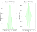 Real and imaginary parts of integrand for Fourier transform at 3 hertz
 -
 Real and imaginary parts of integrand for Fourier transform at 5 hertz
 -
 Fourier transform with 3 and 5 hertz labeled.


Properties of the Fourier transform[editar | editar código-fonte]
An integrable function is a function ƒ on the real line that is Lebesgue-measurable and satisfies

Basic properties[editar | editar código-fonte]
Given integrable functions f(x), g(x), and h(x) denote their Fourier transforms by , , and respectively. The Fourier transform has the following basic properties (Pinsky 2002).


- Linearity
- For any complex numbers a and b, if h(x) = aƒ(x) + bg(x), then
- Translation
- For any real number x0, if h(x) = ƒ(x − x0), then
- Modulation
- For any real number ξ0, if h(x) = e2πixξ0ƒ(x), then .
- Scaling
- For all non-zero real numbers a, if h(x) = ƒ(ax), then . The case a = −1 leads to the time-reversal property, which states: if h(x) = ƒ(−x), then .
- Conjugation
- If , then
- Convolution
- If , then


Uniform continuity and the Riemann-Lebesgue lemma[editar | editar código-fonte]

.svg)
The Fourier transform of integrable functions have additional properties that do not always hold. The Fourier transform of integrable functions ƒ are uniformly continuous and (Katznelson 1976). The Fourier transform of integrable functions also satisfy the Riemann-Lebesgue lemma which states that (Stein & Weiss 1971)


The Fourier transform of an integrable function ƒ is bounded and continuous, but need not be integrable – for example, the Fourier transform of the rectangular function, which is a step function (and hence integrable) is the sinc function, which is not Lebesgue integrable, though it does have an improper integral: one has an analog to the alternating harmonic series, which is a convergent sum but not absolutely convergent.
It is not possible in general to write the inverse transform as a Lebesgue integral. However, when both ƒ and are integrable, the following inverse equality holds true for almost every x:

Almost everywhere, ƒ is equal to the continuous function given by the right-hand side. If ƒ is given as continuous function on the line, then equality holds for every x.
A consequence of the preceding result is that the Fourier transform is injective on L1(R).
The Plancherel theorem and Parseval's theorem[editar | editar código-fonte]
Let f(x) and g(x) be integrable, and let and be their Fourier transforms. If f(x) and g(x) are also square-integrable, then we have Parseval's theorem (Rudin 1987, p. 187):

where the bar denotes complex conjugation.
The Plancherel theorem, which is equivalent to Parseval's theorem, states (Rudin 1987, p. 186):

The Plancherel theorem makes it possible to define the Fourier transform for functions in L2(R), as described in Generalizations below. The Plancherel theorem has the interpretation in the sciences that the Fourier transform preserves the energy of the original quantity. It should be noted that depending on the author either of these theorems might be referred to as the Plancherel theorem or as Parseval's theorem.
See Pontryagin duality for a general formulation of this concept in the context of locally compact abelian groups.
Poisson summation formula[editar | editar código-fonte]
The Poisson summation formula provides a link between the study of Fourier transforms and Fourier Series. Given an integrable function ƒ we can consider the periodization of ƒ given by

where the summation is taken over the set of all integers k. The Poisson summation formula relates the Fourier series of to the Fourier transform of ƒ. Specifically it states that the Fourier series of is given by:


Convolution theorem[editar | editar código-fonte]
The Fourier transform translates between convolution and multiplication of functions. If ƒ(x) and g(x) are integrable functions with Fourier transforms and respectively, and if the convolution of ƒ and g exists and is absolutely integrable, then the Fourier transform of the convolution is given by the product of the Fourier transforms and (under other conventions for the definition of the Fourier transform a constant factor may appear).
This means that if:

where ∗ denotes the convolution operation, then:
In linear time invariant (LTI) system theory, it is common to interpret g(x) as the impulse response of an LTI system with input ƒ(x) and output h(x), since substituting the unit impulse for ƒ(x) yields h(x) = g(x). In this case, represents the frequency response of the system.
Conversely, if ƒ(x) can be decomposed as the product of two square integrable functions p(x) and q(x), then the Fourier transform of ƒ(x) is given by the convolution of the respective Fourier transforms and .


Cross-correlation theorem[editar | editar código-fonte]
In an analogous manner, it can be shown that if h(x) is the cross-correlation of ƒ(x) and g(x):

then the Fourier transform of h(x) is:

Eigenfunctions[editar | editar código-fonte]
One important choice of an orthonormal basis for L2(R) is given by the Hermite functions

where are the "probabilist's" Hermite polynomials, defined by Hn(x) = (−1)nexp(x2/2) Dn exp(−x2/2). Under this convention for the Fourier transform, we have that


In other words, the Hermite functions form a complete orthonormal system of eigenfunctions for the Fourier transform on L2(R) (Pinsky 2002). However, this choice of eigenfunctions is not unique. There are only four different eigenvalues of the Fourier transform (±1 and ±i) and any linear combination of eigenfunctions with the same eigenvalue gives another eigenfunction. As a consequence of this, it is possible to decompose L2(R) as a direct sum of four spaces H0, H1, H2, and H3 where the Fourier transform acts on Hk simply by multiplication by ik. This approach to define the Fourier transform is due to N. Wiener (Duoandikoetxea 2001). The choice of Hermite functions is convenient because they are exponentially localized in both frequency and time domains, and thus give rise to the fractional Fourier transform used in time-frequency analysis {{carece de fontes}}.
Fourier transform on Euclidean space[editar | editar código-fonte]
The Fourier transform can be in any arbitrary number of dimensions n. As with the one-dimensional case there are many conventions, for an integrable function ƒ(x) this article takes the definition:

where x and ξ are n-dimensional vectors, and x · ξ is the dot product of the vectors. The dot product is sometimes written as .

All of the basic properties listed above hold for the n-dimensional Fourier transform, as do Plancherel's and Parseval's theorem. When the function is integrable, the Fourier transform is still uniformly continuous and the Riemann-Lebesgue lemma holds. (Stein & Weiss 1971)
Uncertainty principle[editar | editar código-fonte]
Generally speaking, the more concentrated f(x) is, the more spread out its Fourier transform must be. In particular, the scaling property of the Fourier transform may be seen as saying: if we "squeeze" a function in x, its Fourier transform "stretches out" in ξ. It is not possible to arbitrarily concentrate both a function and its Fourier transform.
The trade-off between the compaction of a function and its Fourier transform can be formalized in the form of an Uncertainty Principle, and is formalized by viewing a function and its Fourier transform as conjugate variables with respect to the symplectic form on the time–frequency domain: from the point of view of the linear canonical transformation, the Fourier transform is rotation by 90° in the time–frequency domain, and preserves the symplectic form.
Suppose ƒ(x) is an integrable and square-integrable function. Without loss of generality, assume that ƒ(x) is normalized:

It follows from the Plancherel theorem that is also normalized.
The spread around x = 0 may be measured by the dispersion about zero (Pinsky 2002) defined by

In probability terms, this is the second moment of about zero.

The Uncertainty principle states that, if ƒ(x) is absolutely continuous and the functions x·ƒ(x) and ƒ′(x) are square integrable, then
- (Pinsky 2002).

The equality is attained only in the case (hence ) where σ > 0 is arbitrary and C1 is such that ƒ is L2–normalized (Pinsky 2002). In other words, where ƒ is a (normalized) Gaussian function, centered at zero.


In fact, this inequality implies that:

for any in R (Stein & Shakarchi 2003).

In quantum mechanics, the momentum and position wave functions are Fourier transform pairs, to within a factor of Planck's constant. With this constant properly taken into account, the inequality above becomes the statement of the Heisenberg uncertainty principle (Stein & Shakarchi 2003).
Spherical harmonics[editar | editar código-fonte]
Let the set of homogeneous harmonic polynomials of degree k on Rn be denoted by Ak. The set Ak consists of the solid spherical harmonics of degree k. The solid spherical harmonics play a similar role in higher dimensions to the Hermite polynomials in dimensions one. Specifically, if f(x) = e−π|x|2P(x) for some P(x) in Ak, then . Let the set Hk be the closure in L2(Rn) of linear combinations of functions of the form f(|x|)P(x) where P(x) is in Ak. The space L2(Rn) is then a direct sum of the spaces Hk and the Fourier transform maps each space Hk to itself and is possible to characterize the action of the Fourier transform on each space Hk (Stein & Weiss 1971). Let ƒ(x) = ƒ0(|x|)P(x) (with P(x) in Ak), then where


Here J(n + 2k − 2)/2 denotes the Bessel function of the first kind with order (n + 2k − 2)/2. When k = 0 this gives a useful formula for the Fourier transform of a radial function (Grafakos 2004).
Restriction problems[editar | editar código-fonte]
In higher dimensions it becomes interesting to study restriction problems for the Fourier transform. The Fourier transform of an integrable function is continuous and the restriction of this function to any set is defined. But for a square-integrable function the Fourier transform could be a general class of square integrable functions. As such, the restriction of the Fourier transform of an L2(Rn) function cannot be defined on sets of measure 0. It is still an active area of study to understand restriction problems in Lp for 1 < p < 2. Surprisingly, it is possible in some cases to define the restriction of a Fourier transform to a set S, provided S has non-zero curvature. The case when S is the unit sphere in Rn is of particular interest. In this case the Tomas-Stein restriction theorem states that the restriction of the Fourier transform to the unit sphere in Rn is a bounded operator on Lp provided 1 ≤ p ≤ (2n + 2) / (n + 3).
One notable difference between the Fourier transform in 1 dimension versus higher dimensions concerns the partial sum operator. Consider an increasing collection of measurable sets ER indexed by R ∈ (0,∞): such as balls of radius R centered at the origin, or cubes of side 2R. For a given integrable function ƒ, consider the function ƒR defined by:

Suppose in addition that ƒ is in Lp(Rn). For n = 1 and 1 < p < ∞, if one takes ER = (−R, R), then ƒR converges to ƒ in Lp as R tends to infinity, by the boundedness of the Hilbert transform. Naively one may hope the same holds true for n > 1. In the case that ER is taken to be a cube with side length R, then convergence still holds. Another natural candidate is the Euclidean ball ER = {ξ : |ξ| < R}. In order for this partial sum operator to converge, it is necessary that the multiplier for the unit ball be bounded in Lp(Rn). For n ≥ 2 it is a celebrated theorem of Charles Fefferman that the multiplier for the unit ball is never bounded unless p = 2 (Duoandikoetxea 2001). In fact, when p ≠ 2, this shows that not only may ƒR fail to converge to ƒ in Lp, but for some functions ƒ ∈ Lp(Rn), ƒR is not even an element of Lp.
Generalizations[editar | editar código-fonte]
Fourier transform on other function spaces[editar | editar código-fonte]
It is possible to extend the definition of the Fourier transform to other spaces of functions. Since compactly supported smooth functions are integrable and dense in L2(R), the Plancherel theorem allows us to extend the definition of the Fourier transform to general functions in L2(R) by continuity arguments. Further : L2(R) → L2(R) is a unitary operator (Stein & Weiss 1971, Thm. 2.3). Many of the properties remain the same for the Fourier transform. The Hausdorff-Young inequality can be used to extend the definition of the Fourier transform to include functions in Lp(R) for 1 ≤ p ≤ 2. Unfortunately, further extensions become more technical. The Fourier transform of functions in Lp for the range 2 < p < ∞ requires the study of distributions (Katznelson 1976). In fact, it can be shown that there are functions in Lp with p>2 so that the Fourier transform is not defined as a function (Stein & Weiss 1971).

Fourier–Stieltjes transform[editar | editar código-fonte]
The Fourier transform of a finite Borel measure μ on Rn is given by (Pinsky 2002):

This transform continues to enjoy many of the properties of the Fourier transform of integrable functions. One notable difference is that the Riemann-Lebesgue lemma fails for measures (Katznelson 1976). In the case that dμ = ƒ(x) dx, then the formula above reduces to the usual definition for the Fourier transform of ƒ.
The Fourier transform may be used to give a characterization of continuous measures. Bochner's theorem characterizes which functions may arise as the Fourier-Stieltjes transform of a measure (Katznelson 1976).
Furthermore, the Dirac delta function is not a function but it is a finite Borel measure. Its Fourier transform is a constant function (whose specific value depends upon the form of the Fourier transform used).
Tempered distributions[editar | editar código-fonte]
The Fourier transform maps the space of Schwartz functions to itself, and gives a homeomorphism of the space to itself (Stein & Weiss 1971). Because of this it is possible to define the Fourier transform of tempered distributions. These include all the integrable functions mentioned above and have the added advantage that the Fourier transform of any tempered distribution is again a tempered distribution.
The following two facts provide some motivation for the definition of the Fourier transform of a distribution. First let ƒ and g be integrable functions, and let and be their Fourier transforms respectively. Then the Fourier transform obeys the following multiplication formula (Stein & Weiss 1971),


Secondly, every integrable function ƒ defines a distribution Tƒ by the relation
- for all Schwartz functions φ.

In fact, given a distribution T, we define the Fourier transform by the relation
- for all Schwartz functions φ.

It follows that .

Distributions can be differentiated and the above mentioned compatibility of the Fourier transform with differentiation and convolution remains true for tempered distributions.
Locally compact abelian groups[editar | editar código-fonte]
The Fourier transform may be generalized to any locally compact Abelian group. A locally compact abelian group is an abelian group which is at the same time a locally compact Hausdorff topological space so that the group operations are continuous. If G is a locally compact abelian group, it has a translation invariant measure μ, called Haar measure. For a locally compact abelian group G it is possible to place a topology on the set of characters so that is also a locally compact abelian group. For a function ƒ in L1(G) it is possible to define the Fourier transform by (Katznelson 1976):


Locally compact Hausdorff space[editar | editar código-fonte]
The Fourier transform may be generalized to any locally compact Hausdorff space, which recovers the topology but loses the group structure.
Given a locally compact Hausdorff topological space X, the space A=C0(X) of continuous complex-valued functions on X which vanish at infinity is in a natural way a commutative C*-algebra, via pointwise addition, multiplication, complex conjugation, and with norm as the uniform norm. Conversely, the characters of this algebra A, denoted are naturally a topological space, and can be identified with evaluation at a point of x, and one has an isometric isomorphism In the case where X=R is the real line, this is exactly the Fourier transform.


Non-abelian groups[editar | editar código-fonte]
The Fourier transform can also be defined for functions on a non-abelian group, provided that the group is compact. Unlike the Fourier transform on an abelian group, which is scalar-valued, the Fourier transform on a non-abelian group is operator-valued (Hewitt & Ross 1971, Chapter 8). The Fourier transform on compact groups is a major tool in representation theory (Knapp 2001) and non-commutative harmonic analysis.
Let G be a compact Hausdorff topological group. Let Σ denote the collection of all isomorphism classes of finite-dimensional irreducible unitary representations, along with a definite choice of representation U(σ) on the Hilbert space Hσ of finite dimension dσ for each σ ∈ Σ. If μ is a finite Borel measure on G, then the Fourier–Stieltjes transform of μ is the operator on Hσ defined by

where is the complex-conjugate representation of U(σ) acting on Hσ. As in the abelian case, if μ is absolutely continuous with respect to the left-invariant probability measure λ on G, then it is represented as


for some ƒ ∈ L1(λ). In this case, one identifies the Fourier transform of ƒ with the Fourier–Stieltjes transform of μ.
The mapping defines an isomorphism between the Banach space M(G) of finite Borel measures (see rca space) and a closed subspace of the Banach space C∞(Σ) consisting of all sequences E = (Eσ) indexed by Σ of (bounded) linear operators Eσ : Hσ → Hσ for which the norm


is finite. The "convolution theorem" asserts that, furthermore, this isomorphism of Banach spaces is in fact an isomorphism of C* algebras into a subspace of C∞(Σ), in which M(G) is equipped with the product given by convolution of measures and C∞(Σ) the product given by multiplication of operators in each index σ.
The generalization of the Fourier transform to the noncommutative situation has also in part contributed to the development of noncommutative geometry.{{carece de fontes}} In this context, a categorical generalization of the Fourier transform to noncommutative groups is Tannaka-Krein duality, which replaces the group of characters with the category of representations. However, this loses the connection with harmonic functions.
Alternatives[editar | editar código-fonte]
In signal processing terms, a function (of time) is a representation of a signal with perfect time resolution, but no frequency information, while the Fourier transform has perfect frequency resolution, but no time information: the magnitude of the Fourier transform at a point is how much frequency content there is, but location is only given by phase (argument of the Fourier transform at a point), and standing waves are not localized in time – a sine wave continues out to infinity, without decaying. This limits the usefulness of the Fourier transform for analyzing signals that are localized in time, notably transients, or any signal of finite extent.
As alternatives to the Fourier transform, in time-frequency analysis, one uses time-frequency transforms to represent signals in a form that has some time information and some frequency information – by the uncertainty principle, there is a trade-off between these. These can be generalizations of the Fourier transform, such as the short-time Fourier transform or fractional Fourier transform, or can use different functions to represent signals, as in wavelet transforms and chirplet transforms, with the wavelet analog of the (continuous) Fourier transform being the continuous wavelet transform.
Applications[editar | editar código-fonte]
Analysis of differential equations[editar | editar código-fonte]
Fourier transforms, and the closely related Laplace transforms are widely used in solving differential equations. The Fourier transform is compatible with differentiation in the following sense: if f(x) is a differentiable function with Fourier transform , then the Fourier transform of its derivative is given by . This can be used to transform differential equations into algebraic equations. Note that this technique only applies to problems whose domain is the whole set of real numbers. By extending the Fourier transform to functions of several variables partial differential equations with domain Rn can also be translated into algebraic equations.

NMR and MR Imaging experiments[editar | editar código-fonte]
Fourier transforms, are also related to the acquisition of a signal in Nuclear Magnetic resonance. Upon aquiring the FID (Free Inductive Decay) an exponential FID signal in the time domain is Fourier transformed to produce a Lorentzian signal in the frequency domain. Furthermore Fourier transforms are also used in MRI experiments where the K-space (the reciprocal space vector) is encoded in the x and y direction, in which the spacial information in the K-space is frequency and phase encoded, respectively. This spatial information which produces an FID from the spinning nuclei is then Fourier transformed to form an image in real space.
Domain and range of the Fourier transform[editar | editar código-fonte]
It is often desirable to have the most general domain for the Fourier transform as possible. The definition of Fourier transform as an integral naturally restricts the domain to the space of integrable functions. Unfortunately, there is no simple characterizations of which functions are Fourier transforms of integrable functions (Stein & Weiss 1971). It is possible to extend the domain of the Fourier transform in various ways, as discussed in generalizations above. The following list details some of the more common domains and ranges on which the Fourier transform is defined.
- The space of Schwartz functions is closed under the Fourier transform. Schwartz functions are rapidly decaying functions and do not include all functions which are relevant for the Fourier transform. More details may be found in (Stein & Weiss 1971).
- The space Lp maps into the space Lq, where 1/p + 1/q = 1 and 1 ≤ p ≤ 2 (Hausdorff–Young inequality).
- In particular, the space L2 is closed under the Fourier transform, but here the Fourier transform is no longer defined by integration.
- The space L1 of Lebesgue integrable functions maps into C0, the space of continuous functions that tend to zero at infinity – not just into the space of bounded functions (the Riemann–Lebesgue lemma).

- The set of tempered distributions is closed under the Fourier transform. Tempered distributions are also a form of generalization of functions. It is in this generality that one can define the Fourier transform of objects like the Dirac comb.
Other notations[editar | editar código-fonte]
Other common notations for are: , , , , , , and Though less commonly other notations are used. Denote the Fourier transform by a capital letter corresponding to the letter of function being transformed (such as f(x) and F(ξ)) is especially common in the sciences and engineering. In electronics, the omega (ω) is often used instead of ξ due to its interpretation as angular frequency, sometimes it is written as F(jω), where j is the imaginary unit, to indicate its relationship with the Laplace transform, and sometimes it is replaced with 2πf in order to use common frequency.


The interpretation of the complex function may be aided by expressing it in polar coordinate form: in terms of the two real functions A(ξ) and φ(ξ) where:


is the amplitude and

is the phase (see arg function).
Then the inverse transform can be written:

which is a recombination of all the frequency components of ƒ(x). Each component is a complex sinusoid of the form e2πixξ whose amplitude is A(ξ) and whose initial phase angle (at x = 0) is φ(ξ).
The Fourier transform may be thought of as a mapping on function spaces. This mapping is here denoted and is used to denote the Fourier transform of the function f. This mapping is linear, which means that can also be seen as a linear transformation on the function space and implies that the standard notation in linear algebra of applying a linear transformation to a vector (here the function f) can be used to write instead of . Since the result of applying the Fourier transform is again a function, we can be interested in the value of this function evaluated at the value ξ for its variable, and this is denoted either as or as . Notice that in the former case, it is implicitly understood that is applied first to f and then the resulting function is evaluated at ξ, not the other way around.


In mathematics and various applied sciences it is often necessary to distinguish between a function f and the value of f when its variable equals x, denoted f(x). This means that a notation like formally can be interpreted as the Fourier transform of the values of f at x. Despite this flaw, the previous notation appears frequently, often when a particular function or a function of a particular variable is to be transformed. For example, is sometimes used to express that the Fourier transform of a rectangular function is a sinc function, or is used to express the shift property of the Fourier transform. Notice, that the last example is only correct under the assumption that the transformed function is a function of x, not of x0.


Other conventions[editar | editar código-fonte]
There are three common conventions for defining the Fourier transform. The Fourier transform is often written in terms of angular frequency: ω = 2πξ whose units are radians per second.
The substitution ξ = ω/(2π) into the formulas above produces this convention:

Under this convention, the inverse transform becomes:

Unlike the convention followed in this article, when the Fourier transform is defined this way it no longer a unitary transformation on L2(Rn). There is also less symmetry between the formulas for the Fourier transform and its inverse.
Another popular convention is to split the factor of (2π)n evenly between the Fourier transform and its inverse, which leads to definitions:


Under this convention the Fourier transform is again a unitary transformation on L2(Rn). It also restores the symmetry between the Fourier transform and its inverse.
Variations of all three conventions can be created by conjugating the complex-exponential kernel of both the forward and the reverse transform. The signs must be opposites. Other than that, the choice is (again) a matter of convention.
| ordinary frequency ξ (hertz) | unitary |
|
|---|---|---|
| angular frequency ω (rad/s) | non-unitary |
|
| unitary |
|


Tables of important Fourier transforms[editar | editar código-fonte]
The following tables record some closed form Fourier transforms. For functions ƒ(x) , g(x) and h(x) denote their Fourier transforms by , , and respectively. Only the three most common conventions are included.

Functional relationships[editar | editar código-fonte]
The Fourier transforms in this table may be found in (Erdélyi 1954) or the appendix of (Kammler 2000)
| Function | Fourier transform unitary, ordinary frequency |
Fourier transform unitary, angular frequency |
Fourier transform non-unitary, angular frequency |
Remarks | |
|---|---|---|---|---|---|
|
|
|
||||
| 101 | Linearity | ||||
| 102 | Shift in time domain | ||||
| 103 | Shift in frequency domain, dual of 102 | ||||
| 104 | If is large, then is concentrated around 0 and spreads out and flattens. | ||||
| 105 | Here needs to be calculated using the same method as Fourier transform column. Results from swapping "dummy" variables of and . | ||||
| 106 | |||||
| 107 | This is the dual of 106 | ||||
| 108 | The notation denotes the convolution of and — this rule is the convolution theorem | ||||
| 109 | This is the dual of 108 | ||||
| 110 | For a purely real even function | , and are purely real even functions. | |||
| 111 | For a purely real odd function | , and are purely imaginary odd functions. | |||


Square-integrable functions[editar | editar código-fonte]
The Fourier transforms in this table may be found in (Campbell & Foster 1948), (Erdélyi 1954), or the appendix of (Kammler 2000)
| Function | Fourier transform unitary, ordinary frequency |
Fourier transform unitary, angular frequency |
Fourier transform non-unitary, angular frequency |
Remarks | |
|---|---|---|---|---|---|
|
|
|
|
|||
| 201 | The rectangular pulse and the normalized sinc function, here defined as sinc(x) = sin(πx)/(πx) | ||||
| 202 | Dual of rule 201. The rectangular function is an ideal low-pass filter, and the sinc function is the non-causal impulse response of such a filter. | ||||
| 203 | The function tri(x) is the triangular function | ||||
| 204 | Dual of rule 203. | ||||
| 205 | The function u(x) is the Heaviside unit step function and a>0. | ||||
| 206 | This shows that, for the unitary Fourier transforms, the Gaussian function exp(−αx2) is its own Fourier transform for some choice of α. For this to be integrable we must have Re(α)>0. | ||||
| 207 | For a>0. | ||||
| 208 |
|
|
|
The functions Jn (x) are the n-th order Bessel functions of the first kind. The functions Un (x) are the Chebyshev polynomial of the second kind. See 315 and 316 below. | |
| 209 | Hyperbolic secant is its own Fourier transform |


Distributions[editar | editar código-fonte]
The Fourier transforms in this table may be found in (Erdélyi 1954) or the appendix of (Kammler 2000)
| Function | Fourier transform unitary, ordinary frequency |
Fourier transform unitary, angular frequency |
Fourier transform non-unitary, angular frequency |
Remarks | |
|---|---|---|---|---|---|
|
|
|
|
|||
| 301 | The distribution δ(ξ) denotes the Dirac delta function. | ||||
| 302 | Dual of rule 301. | ||||
| 303 | This follows from 103 and 301. | ||||
| 304 | This follows from rules 101 and 303 using Euler's formula: | ||||
| 305 | This follows from 101 and 303 using | ||||
| 306 | |||||
| 307 | |||||
| 308 | Here, n is a natural number and is the n-th distribution derivative of the Dirac delta function. This rule follows from rules 107 and 301. Combining this rule with 101, we can transform all polynomials. | ||||
| 309 | Here sgn(ξ) is the sign function. Note that 1/x is not a distribution. It is necessary to use the Cauchy principal value when testing against Schwartz functions. This rule is useful in studying the Hilbert transform. | ||||
| 310 | Generalization of rule 309. | ||||
| 311 | |||||
| 312 | The dual of rule 309. This time the Fourier transforms need to be considered as Cauchy principal value. | ||||
| 313 | The function u(x) is the Heaviside unit step function; this follows from rules 101, 301, and 312. | ||||
| 314 | This function is known as the Dirac comb function. This result can be derived from 302 and 102, together with the fact that as distributions. | ||||
| 315 | The function J0(x) is the zeroth order Bessel function of first kind. | ||||
| 316 | This is a generalization of 315. The function Jn(x) is the n-th order Bessel function of first kind. The function Tn(x) is the Chebyshev polynomial of the first kind. |


Two-dimensional functions[editar | editar código-fonte]
| Function | Fourier transform unitary, ordinary frequency |
Fourier transform unitary, angular frequency |
Fourier transform non-unitary, angular frequency |
Remarks | |
|---|---|---|---|---|---|
|
|
|
|
The variables ξx, ξy, ωx, ωy, νx and νy are real numbers. The integrals are taken over the entire plane. | ||
| 401 | Both functions are Gaussians, which may not have unit volume. | ||||
| 402 | The function is defined by circ(r)=1 0≤r≤1, and is 0 otherwise. This is the Airy distribution and is expressed using J1 (the order 1 Bessel function of the first kind). (Stein & Weiss 1971, Thm. IV.3.3) |


Formulas for general n-dimensional functions[editar | editar código-fonte]
| Function | Fourier transform unitary, ordinary frequency |
Fourier transform unitary, angular frequency |
Fourier transform non-unitary, angular frequency |
Remarks | |
|---|---|---|---|---|---|
|
|
|
||||
| 501 | The function χ[0,1] is the characteristic function of the interval [0,1]. The function Γ(x) is the gamma function. The function Jn/2 + δ a Bessel function of the first kind with order n/2+δ. Taking n = 2 and δ = 0 produces 402. (Stein & Weiss 1971, Thm. 4.13) |


![{\displaystyle \chi _{[0,1]}(|x|)(1-|x|^{2})^{\delta }}](https://wikimedia.org/api/rest_v1/media/math/render/svg/ef6be502ec3070c46594f0d1a08010f01eef0786)


See also[editar | editar código-fonte]
References[editar | editar código-fonte]
- Bochner S.,Chandrasekharan K. (1949). Fourier Transforms. [S.l.]: Princeton University Press
- Bracewell, R. N. (2000), The Fourier Transform and Its Applications 3rd ed. , Boston: McGraw-Hill.
- Campbell, George; Foster, Ronald (1948), Fourier Integrals for Practical Applications, New York: D. Van Nostrand Company, Inc..
- Duoandikoetxea, Javier (2001), Fourier Analysis, ISBN 0-8218-2172-5, American Mathematical Society.
- Dym, H; McKean, H (1985), Fourier Series and Integrals, ISBN 978-0122264511, Academic Press.
- Erdélyi, Arthur, ed. (1954), Tables of Integral Transforms, 1, New Your: McGraw-Hill
- Grafakos, Loukas (2004), Classical and Modern Fourier Analysis, ISBN 0-13-035399-X, Prentice-Hall.
- Hewitt, Edwin; Ross, Kenneth A. (1970), Abstract harmonic analysis. Vol. II: Structure and analysis for compact groups. Analysis on locally compact Abelian groups, Die Grundlehren der mathematischen Wissenschaften, Band 152, Berlin, New York: Springer-Verlag, MR0262773.
- Hörmander, L. (1976), Linear Partial Differential Operators, Volume 1, ISBN 978-3540006626, Springer-Verlag.
- James, J.F. (2002), A Student's Guide to Fourier Transforms, ISBN 0-521-00428-4 2nd ed. , New York: Cambridge University Press.
- Kaiser, Gerald (1994), A Friendly Guide to Wavelets, ISBN 0-8176-3711-7, Birkhäuser
- Kammler, David (2000), A First Course in Fourier Analysis, ISBN 0-13-578782-3, Prentice Hall
- Katznelson, Yitzhak (1976), An introduction to Harmonic Analysis, ISBN 0-486-63331-4, Dover
- Knapp, Anthony W. (2001), Representation Theory of Semisimple Groups: An Overview Based on Examples, ISBN 978-0-691-09089-4, Princeton University Press
- Pinsky, Mark (2002), Introduction to Fourier Analysis and Wavelets, ISBN 0-534-37660-6, Brooks/Cole
- Polyanin, A. D.; Manzhirov, A. V. (1998), Handbook of Integral Equations, ISBN 0-8493-2876-4, Boca Raton: CRC Press.
- Rudin, Walter (1987), Real and Complex Analysis, ISBN 0-07-100276-6 Third ed. , Singapore: McGraw-Hill Parâmetro desconhecido
|publilsher=ignorado (ajuda). - Stein, Elias; Shakarchi, Rami (2003), Fourier Analysis: An introduction, ISBN 0-691-11384-X, Princeton University Press.
- Stein, Elias; Weiss, Guido (1971), Introduction to Fourier Analysis on Euclidean Spaces, ISBN 978-0-691-08078-9, Princeton, N.J.: Princeton University Press Parâmetro desconhecido
|publilsher=ignorado (ajuda). - Wilson, R. G. (1995), Fourier Series and Optical Transform Techniques in Contemporary Optics, ISBN 0471303577, New York: Wiley Parâmetro desconhecido
|publilsher=ignorado (ajuda). - Yosida, K. (1968), Functional Analysis, ISBN 3-540-58654-7, Springer-Verlag.
External links[editar | editar código-fonte]
- Fourier Series Applet (Tip: drag magnitude or phase dots up or down to change the wave form).
- Tables of Integral Transforms at EqWorld: The World of Mathematical Equations.
- Weisstein, Eric W. «Fourier Transform» (em inglês). MathWorld
- Fourier Transform Module by John H. Mathews
- The DFT “à Pied”: Mastering The Fourier Transform in One Day at The DSP Dimension
Category:Fundamental physics concepts Category:Fourier analysis Category:Integral transforms Category:Unitary operators Category:Joseph Fourier pt:Transformada de Fourier
In physics, the zero-point energy is the lowest possible energy that a quantum mechanical physical system may have and is the energy of the ground state. The quantum mechanical system that encapsulates this energy is the zero-point field. The concept was first proposed by Albert Einstein and Otto Stern in 1913. The term "zero-point energy" is a calque of the German Nullpunktenergie. All quantum mechanical systems have a zero-point energy. The term arises commonly in reference to the ground state of the quantum harmonic oscillator and its null oscillations.
Zero-point energy is sometimes used as a synonym for the vacuum energy, an amount of energy associated with the vacuum of empty space. In cosmology, the vacuum energy is one possible explanation for the cosmological constant.[1][2][3] The variation in zero-point energy as the boundaries of a region of vacuum move leads to the Casimir effect, which is observable in nanoscale devices.
A related term is zero-point field, which is the lowest energy state of a field; i.e. its ground state, which is non-zero.[4]
History[editar | editar código-fonte]
In the year 1900, Max Planck derived the formula for the energy of a single "energy radiator", i.e. a vibrating atomic unit, as:

Here, is Planck's constant, is the frequency, k is Boltzmann's constant, and T is the absolute temperature.

In the year 1913, using this formula as a basis, Albert Einstein and Otto Stern published a paper of great significance in which they suggested for the first time the existence of a residual energy that all oscillators have at absolute zero. They called this "residual energy" and then Nullpunktsenergie (in German), which later became translated as zero-point energy. They carried out an analysis of the specific heat of hydrogen gas at low temperature, and concluded that the data are best represented if the vibrational energy is taken to have the form:[5]

According to this expression, an atomic system at absolute zero retains an energy of ½hν.
Foundational physics[editar | editar código-fonte]
The energy of a system is relative, and is defined only in relation to some given state (often called the reference state). One might associate a motionless system with zero energy, but doing so is purely arbitrary. In quantum physics, it is natural to associate the energy with the expectation value of a certain operator, the Hamiltonian of the system. For almost all quantum-mechanical systems, the lowest possible expectation value of this operator, which would be the zero-point energy, is not zero. Adding an arbitrary constant to the Hamiltonian gives an equivalent description of the physical system, but can make the zero-point energy different. Regardless of what constant is added to the Hamiltonian, the minimum momentum is always the same non-zero value.
Varieties[editar | editar código-fonte]
The concept of zero-point energy occurs in a number of situations.
In ordinary quantum mechanics, the zero-point energy is the energy associated with the ground state of the system. The most famous such example is the energy associated with the ground state of the quantum harmonic oscillator. More precisely, the zero-point energy is the expectation value of the Hamiltonian of the system.

In quantum field theory, the fabric of space is visualized as consisting of fields, with the field at every point in space and time being a quantized simple harmonic oscillator, with neighboring oscillators interacting. In this case, one has a contribution of from every point in space, resulting in a calculation of infinite zero-point energy. The zero-point energy is again the expectation value of the Hamiltonian; here, however, the phrase vacuum expectation value is more commonly used, and the energy is called the vacuum energy.
In quantum perturbation theory, it is sometimes said that the contribution of one-loop and multi-loop Feynman diagrams to elementary particle propagators are the contribution of vacuum fluctuations or the zero-point energy to the particle masses.
Experimental observations[editar | editar código-fonte]
A phenomenon that is commonly presented as evidence for the existence of zero-point energy in vacuum is the Casimir effect. This effect was proposed in 1948 by Dutch physicist Hendrik B. G. Casimir (Philips Research), who considered the quantized electromagnetic field between a pair of grounded, neutral metal plates. The vacuum energy contains contributions from all wavelengths, except those excluded by the spacing between plates. As the plates draw together, more wavelengths are excluded and the vacuum energy decreases. The decrease in energy means there must be a force doing work on the plates as they move.[6][7] This force has been measured and found to be in good agreement with the theory. However, there is still some debate on whether vacuum energy explains the Casimir effect as the force can be explained equally well by a different theory involving charge-current interactions (the radiation-reaction picture), as argued by Robert Jaffe of MIT. [8]
The experimentally measured Lamb shift has been argued to be, in part, a zero-point energy effect.[9]
Gravitation and cosmology[editar | editar código-fonte]
Why doesn't the zero-point energy density of the vacuum change with changes in the volume of the universe? And related to that, why doesn't the large constant zero-point energy density of the vacuum cause a large cosmological constant? What cancels it out?
In cosmology, the zero-point energy[10] offers an intriguing possibility for explaining the speculative positive values of the proposed cosmological constant. In brief, if the energy is "really there", then it should exert a gravitational force.[11] In general relativity, mass and energy are equivalent; both produce a gravitational field. One obvious difficulty with this association is that the zero-point energy of the vacuum is absurdly large. Naively, it is infinite, but only differences in energy are physically measurable. The infinity can be removed by renormalization. In all practical calculations, this is how the infinity is handled. It is also arguable that new physics takes over at the Planck scale, and that the energy growth is cut off at that point.[12][13][14][15]
Proposed Free Energy Devices[editar | editar código-fonte]
As a scientific concept, the existence of zero point energy is not controversial although it may be debated. However, perpetual motion machines and other power generating devices supposedly based on zero point energy are highly controversial; although technically zero point energy devices wouldn't hypothetically operate in a closed system, and thereby wouldn't qualify as perpetual motion machines. Descriptions of practical zero point energy devices have thus far lacked cogency. Experimental demonstrations of zero point energy devices have thus far lacked credibility. For reasons such as these, claims to zero point energy devices and great prospects for zero point energy are deemed pseudoscience.
The discovery of zero point energy did not alter the invalidity of perpetual motion machines. Much attention has been given to reputable science suggesting that zero point energy is infinite, but zero point energy is a minimum energy below which a thermodynamic system can never go, thus none of this energy can be withdrawn without altering the system to a different form in which the system has a lower zero point energy. The calculation that underlies the Casimir experiment, a calculation based on the formula predicting infinite vacuum energy, shows the zero point energy of a system consisting of a vacuum between two plates will decrease at a finite rate as the two plates are drawn together. The vacuum energies are predicted to be infinite, but the changes are predicted to be finite. Casimir combined the projected rate of change in zero point energy with the principle of conservation of energy to predict a force on the plates. The predicted force, which is very small and was experimentally measured to be within 5% of its predicted value, is finite.[16] Even though the zero point energy might be infinite, there is no theoretical basis or practical evidence to suggest that infinite amounts of zero point energy are available for use, that zero point energy can be withdrawn for free, or that zero point energy can be used in violation of conservation of energy.[17]
See Also[editar | editar código-fonte]
Fiction
References[editar | editar código-fonte]
- ↑ Florian Bauer(2003)"Zero Point Energy and The Cosmological Constant"
- ↑ James G. Gilson(2007)"Reconciliation of Zero-Point and Dark Energies in a Friedman Dust Universe with Einstein’s Lambda"
- ↑ P. J. E. Peebles and Bharat Ratra(2002)"The Cosmological Constant and Dark Energy"
- ↑ Gribbin, John (1998). Q is for Quantum - An Encyclopedia of Particle Physics. [S.l.]: Touchstone Books. ISBN 0-684-86315-4
- ↑ Laidler, Keith, J. (2001). The World of Physical Chemistry. [S.l.]: Oxford University Press. ISBN 0198559194
- ↑ S.Fabi,B. Harms and G.Karatheodoris(2007)"Zero point energy on extra dimensions: Noncommutative Torus"
- ↑ Guang-jiong Ni"Zero-point energy of vacuum fluctuation as a candidate for dark energy versus a new conjecture of antigravity based on the modified Einstein field equation in general relativity"
- ↑ Jaffe, R. L., Physical Review D. 72, 021301(R) (2005)
- ↑ Margaret Hawton, Self-consistent frequencies of the electron-photon system, Phys. Rev. A 48, 1824 (1993)
- ↑ Barry and Helen Setterfield(2009)"Data and Creation:The ZPE Plasma Model the Science Behind Creation"
- ↑ John R. Ross(2006)"Ross model of the universe"
- ↑ D. Di Mario(2000)"The Black Hole Electron"
- ↑ D. Di Mario(2007)"Magnetic Anomaly in Black Hole Electrons"
- ↑ Paramahamsa Tewari"On the Space-Vortex Structure of the Electron"
- ↑ Alexander Burinskii(2008)"Super black hole as spinning particle: Supersymmetric baglike core"
- ↑ http://math.ucr.edu/home/baez/physics/Quantum/casimir.html - The article refers to an "implied force" from the change in energy, which is the force required by conservation of energy.
- ↑ http://www.sciam.com/article.cfm?id=follow-up-what-is-the-zer
Further reading[editar | editar código-fonte]
- Beiser, Arthur (1967). Concepts of Modern Physics. [S.l.]: McGraw-Hill
- Albert Einstein and L. Hopf (1910). «On a theorem of the probability calculus and its application to the theory of radiation». Ann. Phys. 33: 1096–1104
- Albert Einstein and L. Hopf (1910). «Statistical investigation of a resonator' s motion in a radiation field». Ann. Phys. 33: 1105–1115
- Albert Einstein and Otto Stern, (1913). «—». Ann. Phys. 40. 551 páginas
- Forward, R. (1984). «Extracting electrical energy from the vacuum by cohesion of charged foliated conductors» (PDF). Phys. Rev. B. 30. 1700 páginas. doi:10.1103/PhysRevB.30.1700
- Forward, R. (February 1996). «Mass Modification Experiment Definition». Forward Unlimited. PL-TR-96-3004 Verifique data em:
|data=(ajuda) - Bernard Haisch, Alfonso Rueda and York Dobyns (2001). «Inertial mass and the quantum vacuum fields» (PDF). Annalen der Physik. 10: 393–414. doi:10.1002/1521-3889(200105)10:5<393::AID-ANDP393>3.0.CO;2-Z
- Loudon, R. (2000). The Quantum Theory of Light Third ed. Oxford: Clarendon Press. ISBN 0-19-850176-5
- Milonni, Peter W. (1994). The Quantum Vacuum: an Introduction to Quantum Electrodynamics. New York: Academic. ISBN 0-12-498080-5
- Nernst, W. (1916). «—». Verh. Deutsch Phys. Ges. 18. 83 páginas
- Alfonso Rueda and Bernard Haisch (2005). «Gravity and the Quantum Vacuum Inertia Hypothesis» (PDF). Annalen der Physik. 14: 479–498. doi:10.1002/andp.200510147
- Cook, Nick (2001). The Hunt for Zero Point. London: Century. ISBN 0-7126-69531
- Sciama, D. W. (1991). Simon Saunders and Henry R. Brown, eds, ed. The Philosophy of Vacuum. Oxford: Clarendon Press. ISBN 0-19-824449-5
External links[editar | editar código-fonte]
- Zero-point energy? "Ask the Van" popular science FAQ at University of Illinois.
- Philip Yam, "Exploiting Zero-point Energy", Scientific American Magazine, December 1997, pp. 82-85.
- Matt Visser, What is the 'zero-point energy' (or 'vacuum energy') in quantum physics? Is it really possible that we could harness this energy? from Scientific American Magazine, August 18, 1997
Category:Fundamental physics concepts Category:Energy in physics Category:Fringe physics Category:Quantum field theory Category:Perpetual motion machines pt:Energia de ponto zero
In quantum field theory, the zero-point field is the lowest energy state of a field, i.e. its ground state, which is non zero.[1] This phenomenon gives the quantum vacuum a complex structure, which can be probed experimentally; see, for example, the Casimir effect. The term "zero-point field" is sometimes used as a synonym for the vacuum state of an individual quantized field. The electromagnetic zero-point field is loosely considered as a sea of background electromagnetic energy that fills the vacuum of space. It is often regarded as only a curious outcome of the Heisenberg uncertainty principle measurement problem, which was derived from the fact that the lowest allowable "average" energy level in a harmonic oscillator mode is not zero but ħω/2, where ω is the characteristic angular frequency of the oscillator. However, there is a global scientific consensus developing that the quantized electromagnetic field exists independently of the statistical uncertainty involved in the non-commutative act of measurement, and that it is also fully consistent with changes in the field that are coincident with the act of measurement.
Overview[editar | editar código-fonte]
It is believed that an electromagnetic field exists in a vacuum even when the temperature of the surrounding material is reduced towards absolute zero.[2] The existence of such a zero-point field has been confirmed experimentally by the Casimir experiment, i.e. the measurement of the attractive force between two parallel plates in an evacuated, near-zero temperature enclosure.[2] That force is found to be proportional to the inverse fourth power of the distance apart of the plates; it has been shown that such a result can only be produced by a zero-point field whose spectral energy density has a frequency dependence of ρ(ν) = kν3.[2] It has been assumed until recently, though without any experimental evidence, that there are zero-point energies for the strong and weak forces as well as the electromagnetic force. More recently it has been understood that because the electromagnetic force, expressed by the Lorentz force equation, does not require mass that the electromagnetic zero-point field and the electromagnetic force carrier, the photon, are probably fundamental to all three forces.
History[editar | editar código-fonte]
Quantum mechanics predicts the existence of what are usually called zero-point energies for the strong, the weak and the electromagnetic interactions, where zero-point refers to the energy of the system at temperature T=0, or the lowest quantized energy level of a quantum mechanical system. Specifically, in 1900, Max Planck derived the formula for the energy of a single "energy radiator", i.e. a vibrating atomic unit, as:
- Here, is Planck's constant, is the frequency, k is Boltzmann's constant, and T is the temperature.
In 1913, using this formula as a basis, Albert Einstein and Otto Stern published a paper of great significance in which they suggested for the first time the existence of a residual energy that all oscillators have at absolute zero. They called this "residual energy" and then Nullpunktsenergie (in German), which later became translated as zero-point energy. They carried out an analysis of the specific heat of hydrogen gas at low temperature, and concluded that the data are best represented if the vibrational energy is taken to have the form:[3]
Thus, according to this expression, even at absolute zero the energy of an atomic system has the value ½hν.[4] Although the term zero-point energy applies to all three of these interactions in nature, customarily it is used in reference only to the electromagnetic case.[5] Because the zero-point field has the property of being Lorentz invariant, the zero-point field becomes detectable only when a body is accelerated through space.[5]
Some experiments in 1992 have demonstrated experimentally that the familiar spontaneous emission process in atoms may be regarded as stimulated emission by zero-point field radiation.[6] In recent years, it has been suggested that the electromagnetic zero-point field is not merely an artifact of quantum mechanics, but a real entity with major implications for gravity, astrophysics and technology. This view is shared by a number of researchers, including Boyer (1980), McCrea (1986), Puthoff (1987) and Rueda and Haisch .[7][8][9]
Zero-point energy and conservation of energy[editar | editar código-fonte]
Traditionally it has been assumed that the electromagnetic zpf energy density for each quantum space equals the sum of the quantum oscillatory energy at all possible non-interference producing wavelengths in each of the three spatial dimensions all the way up to the Planck length. Using this historical measure of energy density it has been estimated that there is enough zero point energy contained in one cubic meter of space to boil all of the oceans of the world.
However, the historical analysis of the zpf energy density just described appears to contradict the first law of thermodynamics and our understanding of the cosmology of the universe. The physical evidence is extensive that the universe has expanded from an origin containing essentially no space and infinite energy density in the event called the Big Bang. If our universe is defined as all that has the potential of being known to us and interacted with, then it is defined as a "closed system". A closed system retains causality because its total energy is finite and always conserved. This is not a contradiction with the universe at time (t) = 0 because the concept of infinite energy "density" in "zero" occupied space does not equal "infinite energy" for the universe. The historical analysis of the zpf energy density used in the example of energy in one cubic meter of space does not account for the expansion of the universe. It simply increments this expanding space over time and assigns each new additional quantum space with the maximum energy density.
There is a major drive in physics to create a more realistic zpf energy density model that still allows for causality and conservation of energy in the universe. There is substantial evidence in quantum physics, via the de Broglie relations, the Casimir effect, and the Zitterbewegung action of electrons that this field of energy acts as an energy intermediary in the dynamic actions of all particles. Electrons orbiting a nucleus, as one specific example, may use this energy source to move up in an orbit, and then contribute back to this energy source when they relax back into a lower orbit around the nucleus. The de Broglie relations show that the wavelength is inversely proportional to the momentum of an electron and that the frequency is directly proportional to the electron's kinetic energy. As long as the electron does not increase its average kinetic energy over time through acceleration or heating of the atom as a whole, then this wave-like movement of electrons can be seen as a direct interaction of electrons with the zpf.
A potentially promising area for research is the fact that if particles become more energetic as they are heated or accelerated their gravitational field increases. Changes in gravity can perhaps be attributed to a change in a spherical zpf energy density gradient surrounding an accelerated or decelerated massive particle. This dynamic action is just an extension of the static orbiting electron wave model to a dynamic model in which the "average" kinetic energy of a particle no longer remains constant over time and energy is drawn in from the quantum vacuum but not returned. If a massive particle's ground state is defined as its reference frame at the instant of its creation, then when a particle or body returns to this reference frame, or ground state, from an accelerated state that energy is returned to the quantum vacuum as a decrease in gravity surrounding the particle. This would be in accord with the rules of gravity on accelerated bodies as we know them, and most importantly, maintains conservation of the combined energy of both particles and the zpf, while still allowing for dynamic interaction between the two.
Quantum fluctuations versus quantum pathways[editar | editar código-fonte]
The essential character of the zpf was originally described by John Archibald Wheeler[10] as a foamy sea of constantly emerging virtual particles and anti-particles which would come into existence spontaneously and then annihilate themselves. This description originated because it was the only way to consolidate the enormous projected energy density of the quantum vacuum. Because the mathematics of oscillators was the origin of our understanding of the zpf it has been described as "fluctuating" in the absence of any outside force. But there seems to be a fundamental confusion about this from which subsequent errors in logic arise. An individual oscillator can fluctuate, just as an electron's orbital wave motion can fluctuate between two different orbits, however the "rate" of fluctuation, i.e. a quantum oscillator's characteristic frequency, should never change unless a photon, the electromagnetic force carrier, is either absorbed or emitted by the quantum oscillator. If a point in space could actually be brought to a temperature of zero kelvins the flow of photonic energy between quantum oscillators would stop but each quantum oscillator would still "fluctuate" at a rate that never changes. The energy from one quantum oscillator would not propagate to other quantum spaces. Similarly, at that temperature an electron would maintain its fluctuation between the same two orbits about the nucleus without any change. However from an outside viewpoint the situation would be seen as a static and non-fluctuating one because photons do not escape or enter the quantum space between the two electron orbits.
A static, but plastic quantum foam is a better analogy to the character of the quantum vacuum, and not the kind of "spontaneously" changing foam Wheeler described. It should be remembered that each quantum space represents the sum of quantum harmonic oscillator energy in each of the three spatial degrees of freedom, and that each of these three degrees of freedom can act separately, but in coordination with the other two to provide a total energy for that quantum space which is always conserved. If a photon with a specific energy and direction enters and then exits a quantum space these three degrees of freedom allow for a change in the magnitude of the energy in each of the three spatial directions while conserving the total magnitude of harmonic energy in that space - an increase in magnitude of harmonic energy in one dimension can be compensated by a decrease in the other two dimensions. The orientation and size of these changes will correlate to a change in direction of any particle passing through that quantum space, and to the magnitude, or state of the existing harmonic energy in the three dimensional degrees of freedom for that quantum space at the time the photon enters. Similarly, any particle encountering a quantum space which has recently had a particle pass through it will be affected by that previous particle, even though they are not coincident in time.
For example, in the cold reaches of space between galaxies photons from distant galaxies arrive rarely. If by chance a rare photon passes through one of these cold dark spaces it will leave a quantum signature on the oscillatory energy of each quantum space it passes through. If a quantum space has experienced a photon passing through it and no further photons pass through, then that area of space will retain a memory of the last photon it experienced. That space will then exhibit a residual force which has a magnitude and a direction that resides in the memory of that space. This force can be observed in the Zitterbewegung, or jittery action of electrons, which in principle can be extended to all particles. In effect, a pathway has been produced by this single photon. The fact that this pathway cannot be maintained in its unaltered form after measuring it, as the Heisenberg Uncertainty Principle predicts, does not alter the fact that this pathway is retained in space until the next photon passing through creates an interference with this pathway. Acts of measurement represent an exchange of photons between the "observer" and the "observed" and are synonymous with local changes in energy. The "observed" can be an actual particle or just the pathway in space created by the particle. The appearance of fluctuation is actually the transformation of energy and information as it travels through space, but the total energy and information of the universe are always maintained. So it is seen that this quantum foam is not the kind of foam that springs back, but is more like milk foam on top of a cup of cappuccino - a straw can be pushed through the foam and a hole in the foam will remain for a time after the straw is withdrawn. But in the case of quantum foam the impression left behind is not of a hole, but rather the impression of the photon or particle with mass that passed through it.[11].
Curvature of space and the physical vacuum[editar | editar código-fonte]
Zero-point field theory originated from the application of thermodynamics to the problem of Black Body radiation. This knowledge was later used by Albert Einstein to calculate the electromagnetic residual energy of the vacuum surrounding the electron in the hydrogen atom that was required to keep it from collapsing into the nucleus. Much later the energy density of empty space was calculated to have a spectral density of . This energy density is an enormous figure and is approximately 10120 times higher than the cosmological constant predicts if, as is traditionally done, the Planck length is used for the upper bound for the frequency. The total energy of the universe does not seem to be conserved unless laws of physics are invoked that cannot be understood at the classical level. In other words, the observed expansion of the universe leads to a discrepancy from quantum physics derived vacuum energy of the order of 10120 times. This was originally not seen as a problem because the cosmological constant itself was seen to be on mathematically unfirm ground. It is a positive number very close to zero, but not zero, and it was assumed for many years that this was a mistake and that in actuality it was zero. This assumption came from quantum mechanics which said that virtual particle and anti-particle production and annihilation fluctuations accounted for the large density of the vacuum. In this view an unknown field, or supersymmetric particle system to all known particles, acted as a negative energy source that completely cancelled this energy, just as the cosmological constant should have predicted.

However, the recent red shift observations of type 1a supernovae have illustrated decisively that the universe is accelerating its expansion.[12] This proves that the universe really does have a non-zero vacuum energy. It calls into question the usefulness of the present application of annihilation operators used in quantum mechanics for the current state of the universe. If there really is production and annihilation of virtual particles it must be on a vastly smaller scale than is proposed in the standard model of quantum physics. And any decrease in virtual particle production and annihilation might allow for a lower vacuum energy that would not need to be cancelled. If the vacuum has a finite positive energy then one must find reasons for seeing that reality in the sum of what we observe. One must assume that there are answers to these questions in the observable universe and that we don't understand everything yet. A quantum mechanical fluctuation should occur for a reason, and at a rate that corresponds to the vacuum energy density we currently observe in the universe. One cannot invoke another world or universe to justify unjustifiable fluctuations just when it is useful to solve an inconvenient problem, as in the many worlds philosophy of quantum mechanics.
Geometrodynamics represents the macroscopic curvature of spacetime, but it appears there are more complex forces at work that represent the granularity of space-time around massive particles and bodies. Thus, the famous Russian physicist and political dissident Andrei Sakharov said, "Geometrodynamics is neither as important or as simple as it looks. Do not make it the point of departure in searching for underlying simplicity. Look deeper, at elementary particle physics." Einstein's geometrodynamics, which looks simple, is interpreted by Sakharov as a correction term in particle physics. In this view the cutoff at the Planck length arises purely out of the physics of field and particles, and this governs the value of the Newtonian constant of gravity, G. And the value of the vacuum energy density function with respect to the volume of the universe, , is a constant and is governed by the value of the gravitational constant, G.[13] This energy density does not vary with changes in the volume of the universe because the gravitational constant does not change with the volume of the universe.

Energy in its classical description is a scalar quantity that is always positive. Energy in its particulate form is the photon, and there is no anti-photon. The energy released in the annihilation between matter and anti-matter is in the form of photons. So it may be said that all energy is positive and only in the statistical counterpoint of opposite direction of spin in matter and anti-matter in the Dirac sea can any energy be considered as negative, as opposed to another energy being positive. In addition, because the cosmological constant now has a confirmed small positive energy density the negative energy concept no longer serves a useful purpose in creating a balance of zero observed energy for the universe. Therefore, an effort should be made in physics to erase the idea of negative energy because it violates the first law of thermodynamics and adds a layer of needless confusion. However, removing the concept of negative energy will force a modification to be made to Sakharov's model of energy density, and will even change the idea of the quantum scale energy density of the universe being constant with changes in the volume of the universe. This agrees with the observed temperature of space being lowered as the universe expands, as is reflected in the radiation temperature of the cosmic microwave background radiation. One must now try to find a way to include the mathematical "appearance" of the large constant Planck length vacuum energy density used to support the existence of massive particles, while finding a suitable candidate quantity to subtract from that answer to create a final answer that agrees with the cosmological constant.
The Planck length[editar | editar código-fonte]
It can be noted in that the volume of the universe, , is expanding. If the total energy of the universe is taken as a positive constant based on first principles, then is not a constant throughout the life of the universe - the density gets lower as the volume of the universe expands. However it will be a "changing" constant in the sense that it is an "average" density that applies to the entire universe at any given moment in the life of the universe. It can be safely assumed that if Sakharov was correct in his analysis regarding the defining nature of the gravitational constant, something that is only tentatively accepted as of now, that there is something incorrect in our current mathematical assumptions in physics. If Sakharov's analysis is tentatively taken as true then certain results must accrue from that and other results, long assumed, must be incorrect. The final decision on whether it is worthwhile to accept his analysis is based solely on the utility, or non-utility in finding answers to problems long plagueing physics.

The Planck length defines the shortest wavelength quantum oscillator that is possible. The summation of energy of all possible non-interfering wavelengths for each of the three dimensional degrees of freedom up to this limit has historically defined the energy for each quantum space. And each quantum space is in turn defined as the Planck volume, or .

The Planck length is:

where:
- is the speed of light in a vacuum;
- is the gravitational constant;
- is the reduced Planck constant, the Planck constant divided by 2π.


Perhaps the Planck length is not a constant but stretches out as the universe expands? If the zpf energy density decreases as the volume of the universe expands then, by definition, the changing Planck length would define both the Planck volume and the total energy within each Planck volume. However, this quantum energy/volume relationship should be considered only an average value for the universe at any moment in the life of the universe. There is a precedent for this in the stretching out of light in the cosmic microwave background radiation. When electrons were initially captured in hydrogen atoms in the early universe high energy, short wavelength, photons were released. But in today's universe those wavelengths now appear as much, much longer microwave wavelength photons, but with a distribution and inferred spatial temperature that varies slightly throughout the universe about one unique average value. There are three constants used to create the Planck length constant, as shown above. Is it possible that the gravitational constant, always assumed to be constant throughout the expansion of the universe, is not a constant? This seems plausible, in view of structural changes that would occur in the universe as the fabric of space becomes less dense as it expands. Of the three constants included in the Planck length the gravitational constant seems to be most directly correlated with the expansion of this primordial field.
If one considers fundamentally altering the status of one the three constants then altering the gravitational constant would be preferable to altering the constancy of the speed of light or changing Planck's constant. Planck's constant and the speed of light fundamentally underlie all current calculations of physical properties. Albert Einstein's quantum derivation for the packet of energy in a single photon is:

or for the wavelength, :

Planck's constant is the constant of proportionality in the ratio of the frequency of the photon to the energy of the photon. When the frequency of a photon changes the energy of the photon changes via the constant h. Today the photons in the cosmic microwave background radiation have both lower frequency and subsequently lower energy than when they were originally emitted from hydrogen atoms. Temperature, frequency-wavelength, and especially length, are all time dependent measurements. Time slows down within gravitational fields and it would also slow down within the universe as a whole if the energy density is reduced during its expansion. As the flow of energy and information slows down as the zpf density is reduced within gravitational fields and as the universe expands then these time dependent measurements are all locked together and change together. Just as h is a constant of proportionality between two variables that change together, frequency and energy, c can also be considered a constant of proportionality between two variables that change together, time and length. For a specific object being measured, the direct correlation of change in measurement of distance with the change in measurement of time creates the constancy of the speed of light. This in turn determines the measured wavelength, and thus the temperature of a given object, through Planck's constant. The only constant remaining in the Planck length that is not a result of a time dependent measurement is the gravitational constant, G. This means the only constant that remains available for modification if the average total energy density of the universe "does" change as the universe expands is the gravitational constant. Thus, the gravitational constant, G, is probably not a constant quantity throughout the expansion of the universe. The gravitational constant underlies many of the fundamental properties of physics and the properties affected by the gravitational constant, i.e. the measurement of the dimensions of space and time and temperature, seem to be directly tied to contradictions that already exist between gravitational physics and quantum physics.
Only future experience will tell if more problems are "solved" or if more problems are "created" by allowing for changes in the gravitational constant during the evolution of the universe. One thing is certain though: If the Planck length stretches out as the universe expands then the zpf energy density is not even close to what it is currently assumed to be.
Limits on causality and quantum tunneling[editar | editar código-fonte]
Residual forces can be observed whenever a charge, be it a photon or a massive composite particle, encounters a recent, or not so recent, pathway of a previous particle trajectory. The force it exerts on any charged particle will be:
![{\displaystyle \mathbf {F} =q[\mathbf {E} +(\mathbf {v} \times \mathbf {B} )]}](https://wikimedia.org/api/rest_v1/media/math/render/svg/cb4e83084d7544995ea75f2056b67d6764b49f6d)
The force exerted by these pathways on any test charge will be indistinguishable from a magnetic force because the overwhelming probability is that these paths, relative to the test charge, will be moving in a different inertial reference frame from the test charge. In other words, there will be a relative velocity difference between the test charge and the "ghost particles" that represent the past history of particles in that area of space. But in open space the statistical probability is that these B field zitterbewegung forces will be equal in all directions. Only when the test charge is accelerated from its inertial reference frame will these forces shift to a maximum in the plane normal to the acceleration as the test charge cuts across many more lines of force in that one direction. This counterforce is experienced as inertia to the test charge. The resultant direction imposed on any particle in open space will average out to the initial direction of the force that created the acceleration. However it will be a path combined from connecting many lateral movements that combine to form a helical motion.[14][15]
Just as these forces will impinge on any test charge, this test charge will also affect the oscillatory energy within each quantum space and will modify them according to the magnitude and velocity of the test charge. There will be a balancing of the energy of angular velocity imparted to the particle trajectory with an equal and opposite change in oscillatory energy for the three spatial dimensions. If the trajectory of a charge entering a space does not match the direction of a force currently existing within a quantum space then both the exit trajectory of the test charge and the direction of the force within the quantum space will be altered, as its path integral predicts.[16][17] The exact mechanism creating the change in force is as yet undetermined. It may be a result of just a change in the ratios of oscillatory energy between the three dimensions in a quantum space, while maintaining the same total energy within that quantum space. It may also be a result of a change in total energy within that quantum space in addition to a change in ratios of oscillatory energy in the three dimensions. The problem in determining this would lie in whether or not there is more energy in the charge entering the quantum space than there is total oscillatory energy in all three dimensions in that quantum space before the event occurs. Further mathematical modeling will be required to determine the exact nature of the mechanism under differing circumstances. That resultant force vector can be viewed simultaneously as the energy within a quantum space and also as a barrier between quantum spaces. And any space can be considered a single quantum space if it contains a single force that is continuous in one dimension.
The interesting question to ask is if accelerations can occur that overwhelm the ability of the residual force within a quantum space to modify the trajectory of a particle. It appears possible for a very high energy charge to tunnel through that force and leave the force, or barrier, parallel or nearly parallel, with the original trajectory of the charge. In this way the oscillatory energy in one direction is increased to a level that the energy in the other two dimensions are unable to compensate for it. This can be understood by realizing the oscillatory energy in the other two dimensions cannot be reduced below a value of zero. The totality of space after the tunneling occurs can be considered a larger volume than originally existed if one equates the length of that force in the same way one equated the Planck length3 to the Planck volume. And the seeming non-conservation of energy within this stretched out quantum space is equalized by the same energy dividing into a now larger volume of "combined" spaces. This can be understood because while the oscillatory energy within one quantum space may be increased through the charge tunneling process, the energy from the charge that originally creates that tunneling is simultaneously subtracted from a separate corresponding quantum space. This reduction is reflected in a larger gravitational constant, G, as the expansion proceeds. It is speculated that this is how the universe may have been created in the big bang.
There is a thermodynamic price to pay for this local violation of conservation of energy within a quantum space though. Time is measured by the flow of energy and information as it moves through space. Inertia is caused by the resistance of a test charge to the acceleration as it cuts across more of these lines of force in one direction. Time can also be seen as resistance to the flow of information between distant points in space created by that inertia. But the space between any two distant points between which a charge of overwhelming energy has passed will have a resultant force that is parallel with that path. There will be no inertia to information flow between those two points because there will be no lines of force that have a force component normal to the path between those two points. If a force is imposed on one end of the path it will immediately result in equal and opposite forces imposed on the other end of the path. This is what results in angular momentum in particles with mass. The onset of angular momentum is what creates the division between matter and non-matter, and it also creates the separation between the quantum space from which the photon was taken and the quantum space to which the photon was added. Mass is the energy encapsulated within these rotating pathways that creates the non-local link in composite massive particles.
In reality this tunneling after-effect, or quantum entanglement, is seldom perfect and neither is it evenly distributed in the universe, as can be seen in the WMAP surveys. The lines of force are seldom lined up perfectly parallel to distant points in space. In other words, there can be vast differences in the amount of zpf density, both in spatial distribution and in absolute levels of energy density within any pre-specified average sized volume within the universe, depending on the scale one is looking at. At the quantum scale within fundamental massive particles they "will" be nearly lined up, depending on how long lived they are before they decay. At the cosmic scale it is appearing increasingly likely that there is a similar, but much smaller energy density difference between galaxies and the vast open spaces between the galaxies, because if one mathematically subtracts the gravitational effect of visible matter within each galaxy there is more angular momentum than there should be in the outer reaches of galaxies.
Andrei Sakharov and the elasticity of space[editar | editar código-fonte]
It is a fact that Albert Einstein's equation in General Relativity for the geometrodynamics of space is one of the most beautiful equations in physics. Unfortunately, its beauty has resulted in a fixation in the West on the mathematics of geometry, including the geometry of hyper-dimensional space. This focus has resulted in Western mainstream physics ignoring the need for a mathematical definition that connects the classical General Relativity 4-dimensional and Kaluza-Klein 5-dimensional theories of the geometry of space with new quantum mechanical derived ideas that will better correlate with them. Until an explicit mathematical equation is robustly proven to link these two disparate interpretations of physics the first law of thermodynamics for our universe appears to be conceptually violated.
Andrei Sakharov's conception of the elasticity of space, though incomplete, seems to point towards an ultimate resolution of this problem. In his cosmological model space is elastic like the surface of a balloon and thins out as the volume of the universe expands over time. If the 3-dimensional volume of the universe is represented as a 3-dimensional surface of a balloon, then in its collapsed state at the beginning of time the zpf energy density of the universe is greatest. In approximately the first 10-24 of a second in the life of the universe the zpf energy density would be extremely high, high enough to create the proton in the hydrogen atom. The proton represents approximately 99.9 percent of the mass of the entire hydrogen atom. The estimated energy density of the physical vacuum at the instant of the proton creation would then represent approximately the amount of energy density recently calculated for the hydrogen atom using stochastic electrodynamics.[18] However, in this conceptual framework this zpf energy density would only exist at precisely this one moment in the life of the universe. Sakharov conceived that at the instant of the creation of fundamental massive particles that the elastic zpf energy required for their mass was transformed into inelastic energy.
(Though Sakharov didn't know this when he conceptualized this idea, today our experimental knowledge indicates the proton, which itself is made up of three quarks, is the only fundamental massive particle that does not undergo transformation through radioactive decay if given a long enough time of observation or a large enough quantity of protons being observed. In the case of neutrinos, they simply transform into other kinds of neutrinos. So his idea seems to fit in with the idea of a type of "absolute" inelasticity that the Standard Model cannot account for.)
So a question similar to the question Einstein proposed concerning the non-collapse of the electron into the hydrogen nucleus at zero kelvins can be posed for the proton: Why doesn't the proton radioactively decay if the energy density of the physical vacuum is now a tiny fraction of what it was when the proton was created? The principle of asking why is exactly the same even though they apply to different processes occurring under different conditions, i.e., the relationship of the process to the environmental conditions are similar in both cases. If the zpf energy density decreases over time the statistical probability of the proton decaying should increase. If the proton composes 99.9 percent of the energy of the hydrogen atom, is itself a composite elementary particle, an even more pertinent question would be to ask why the proton doesn't radioactively decay?
Sakharov imagined that spin and its associated angular momentum provided this inelasticity. Spin, and specifically inelastic spin, is a part of a 5-dimensional definition that directly correlates with gravity in Kaluza-Klein theory. If one maintains the balloon metaphor then we sew in a round piece of inelastic material into our balloon at 10-24 seconds into the expansion from its collapsed state. We are careful to select a piece of inelastic material to substitute for the elastic material that has exactly the same density as the same equivalent elastic material surrounding it at that point in its expansion. As we continue to blow up the balloon its elastic material thins out symmetrically except where the inelastic patch is located. Because the area of the inelastic patch does not stretch and thin out the elastic material surrounding it must compensate by stretching and thinning even more than it otherwise would. The greatest thinning will be right on the periphery of the patch in the elastic material because this is the part of the elastic material that has the greatest concentration of stress. If we translate this idea to 3-dimensional vacuum energy physics the greatest zpf stress, or thinning out, will be right on the periphery of any massive body and this is where gravity is greatest.
One now returns to the question of where the missing energy went to that is required to support the proton in today's greatly expanded universe. Using pure logic it appears that the proton still has it in the form of energy pulled in from the surrounding physical vacuum. Though the inelasticity between a proton's quarks can by no means account for all the gravity in the universe it certainly can account for nearly all the gravity of unbound nucleons, i.e., individual protons and neutrons. A neutron can be included in this approximation because it has very slightly more energy than a proton and will decay into a proton after fifteen minutes if separated from protons. It should be remembered that the quarks in protons were bound together though the quantum tunneling mechanism in the overwhelming acceleration of the big bang. And quantum tunneling in the earliest inflationary phase of the expansion of the universe originated from high energy photons overpowering the quantum oscillation energy in a quantum space. The expenditure of energy in the tunneling process resulted in the small bare masses of quarks we see today and the huge binding energy between the three quarks. It is the most significant result of all the results from the inflationary phase of the expansion of the universe.
However, any photons creating a tunneling effect must be accounted for in the quantum space it inhabited before the tunneling took place. Besides the tunneling action creating more space in the universe it also created a deficit, or subtraction of energy from the quantum space each photon inhabited before the tunneling occurred. Gravity seems to be created by that subtraction. This is not gravity as we are used to understanding it, but gravity as a lower energy density gradient in the vacuum spreading out smoothly around any massive object. So it can be seen that the reason the proton does not decay in today's universe is because energy is pulled in from the surrounding physical vacuum. We experience that reduction in energy as gravity.
Related[editar | editar código-fonte]
In recent years, a number of new age books have begun to appear propounding the view that the zero-point field of physics is the secret force of the universe being used to explain such phenomena as intention, remote viewing, paranormal ability, etc.[19][20] One of the main purveyors of this view is Stanford physicist Harold Puthoff who spent more than thirty years examining the zero-point field.[21] Books that promote this view include:
- Lynne McTaggart's 2001 The Field - the Quest for the Secret Force of the Universe.
- Ervin Laszlo's 2004 Science and the Akashic Field - an Integral Theory of Everything.
- Brenda Anderson's 2006 Playing the Quantum Field - How Changing Your Choices Can Change Your Life.
- Masaru Emoto's 2005 "The Hidden Messages in Water."
Such views are not without controversy. Some see such discussion as pseudoscience. [22] However, physicist David Bohm and other respected scientists, have found some utility in looking at the relationship of the zero point field to matter. Bohm posited, for example, that the field might be the force from which all life unfolds. He stated that the "nonlocality" of quantum physics, which could also be described as varying levels of inelasticity between remote points in space, might be explained through interconnections allowable via the zero-point field.
References in popular culture[editar | editar código-fonte]
Though seldom used in fiction, the most notable reference to the Zero-point field is the use of ZPMs in the Stargate universe, devices which extract huge amounts of energy from a Zero-point field. In the video game Half-Life 2, there is also a weapon called the Zero-Point Energy Field Manipulator, more commonly known as the "Gravity Gun". In their 1996 fictional book, Encounter With Tiber, Buzz Aldrin and John Barnes have Alpha Centaurians visit Earth in 7200BC using laserable Zero-Point Field-based propulsion to achieve near-light speed travel. In the 2004 animated film The Incredibles, Syndrome's basic weapon is a zero-point energy field. Saint, a 2006 mystery novel by Ted Dekker, portrays characters who are able manipulate the zero-point field. In Australian author Matthew Reilly's two novels The Six Sacred Stones (2007) and The Five Greatest Warriors (2009), a zero-point field (referred to as the 'Dark Sun') is featured as the threat from which the world requires saving through use of ancient technology and long-lost knowldege.
References[editar | editar código-fonte]
- ↑ Gribbin, John (1998). Q is for Quantum - An Encyclopedia of Particle Physics. [S.l.]: Touchstone Books. ISBN 0-684-86315-4
- ↑ a b c Dodd, John, H. (1991). Atoms and Light: Interactions. [S.l.]: Springer. p. (217). ISBN 0306437414
- ↑ Laidler, Keith, J. (2001). The World of Physical Chemistry. [S.l.]: Oxford University Press. ISBN 0198559194
- ↑ Introduction to Zero-Point Energy - Calphysics Institute
- ↑ a b Zero-point Energy and Zero-point Field – Calphysics Institute
- ↑ S. Haroche and J.-M. Raimond, “Cavity Quantum Electrodynamics,” Sci. Am., pp. 54-62 (April 1993). Also H. Yokoyama, “Physics and Device Applications,” Science 256, pp. 66-70 (1992).
- ↑ Boyer, T.H. (1980). In Foundations of Radiation Theory and Quantum Electrodynamics (ed. Barut, A.O.), Plenum, New York, 49.
- ↑ McCrea, W.H. (1986). Quart. J. Roy. Astr. Soc. 27, 137.
- ↑ Puthoff, H.E. (1987). Phys. Rev. D. 35, 3266.
- ↑ Wheeler, John (1998). Geons, Black Holes, and Quantum Foam: A Life In Physics. [S.l.]: Norton & Company. ISBN 0393319911
- ↑ Habegger, E.J., Quantum Vacuum Pathway Theory, Space Technology and Applications International Forum, (STAIF 2005), AIP Conference Proceedings 746 , 1379.
- ↑ Adam G. Riess et al. (Supernova Search Team) (1998). «Observational evidence from supernovae for an accelerating universe and a cosmological constant» (subscription required). Astronomical J. 116: 1009–38. doi:10.1086/300499
- ↑ Misner, Charles W.; Kip S. Thorne, John Archibald Wheeler (September 1973). Gravitation. San Francisco: W. H. Freeman. ISBN 0-7167-0344-0.
- ↑ B. Haisch, A. Rueda & H.E. Puthoff, (1994). "Inertia as a zero-point-field Lorentz force". Physical Review A, Vol. 49, No. 2, pp. 678-694.
- ↑ Haisch, Bernard; and Rueda, Alfonso (1998). "Contribution to inertial mass by reaction of the vacuum to accelerated motion". Found. Phys. 28: 1057–1108.
- ↑ Feynman, R. P. (1948). "The Space-Time Formulation of Nonrelativistic Quantum Mechanics". "Reviews of Modern Physics" 20: 367–387. doi:10.1103/RevModPhys.20.367
- ↑ Feynman, R. P., and Hibbs, A. R., Quantum Mechanics and Path Integrals, New York: McGraw-Hill, 1965 [ISBN 0-07-020650-3]. The historical reference, written by the inventor of the path integral formulation himself and one of his students.
- ↑ Daniel C. Cole & Yi Zou, "Quantum Mechanical Ground State of Hydrogen Obtained from Classical Electrodynamics", Physics Letters A, Vol. 317, No. 1-2, pp. 14-20 (13 October 2003), quant-ph/0307154 (2003).
- ↑ Brilliant Disguise: Light, Matter and the Zero-Point Field – Bernard Haisch, 2001 Science & Spirit Magazine
- ↑ The Field: The Quest For The Secret Force Of The Universe – Lynne McTaggart, Book Synopsis.
- ↑ McTaggart, Lynne (2007). The Intention Experiment. [S.l.]: Free Press. p. (13). ISBN 0743276957
- ↑ Exploiting Zero-point Energy – Philip Yam, Scientific American Magazine, December 1997, pp. 82-85.

In classical mechanics, a harmonic oscillator is a system which, when displaced from its equilibrium position, experiences a restoring force proportional to the displacement according to Hooke's law:


where is a positive constant.
If is the only force acting on the system, the system is called a simple harmonic oscillator, and it undergoes simple harmonic motion: sinusoidal oscillations about the equilibrium point, with a constant amplitude and a constant frequency (which does not depend on the amplitude).
If a frictional force (damping) proportional to the velocity is also present, the harmonic oscillator is described as a damped oscillator. Depending on the friction coefficient, the system can:
- Oscillate with a frequency smaller than in the non-damped case, and an amplitude decreasing with time (underdamped oscillator).
- Decay exponentially to the equilibrium position, without oscillations (overdamped oscillator).
If an external time dependent force is present, the harmonic oscillator is described as a driven oscillator.
Mechanical examples include pendula (with small angles of displacement), masses connected to springs, and acoustical systems. Other analogous systems include electrical harmonic oscillators such as RLC circuits (see Equivalent systems below). The harmonic oscillator model is very important in physics, because any mass subject to a force in stable equilibrium acts as a harmonic oscillator for small vibrations. Harmonic oscillators occur widely in nature and are exploited in many manmade devices, such as clocks and radio circuits. They are the source of virtually all sinusoidal vibrations and waves.
Simple harmonic oscillator[editar | editar código-fonte]

A simple harmonic oscillator is an oscillator that is neither driven nor damped. Its motion is periodic— repeating itself in a sinusoidal fashion with a constant amplitude, A. Simple harmonic motion SHM can serve as a mathematical model of a variety of motions, such as a pendulum with small amplitudes and a mass on a spring. It also provides the basis of the characterization of more complicated motions through the techniques of Fourier analysis.
In addition to its amplitude, the motion of a simple harmonic oscillator is characterized by its period T, the time for a single oscillation, its frequency f, the reciprocal of the period f = 1/T (i.e. the number of cycles per unit time), and its phase φ, which determines the starting point on the sine wave. The period and frequency are constants determined by the overall system, while the amplitude and phase are determined by the initial conditions (position and velocity) of that system. Overall then, the equation describing simple harmonic motion is
- .

Alternatively a cosine can be used in place of the sine with the phase shifted by π/2.
The general differential force equation for an object of mass m experiencing SHM is:
- ,

where k is the 'spring constant' which relates the displacement of the object to the force applied to the object. The general solutions of this equation is given above with the frequency of the oscillations given by:
- .


The velocity and acceleration of a simple harmonic oscillator oscillate with the same frequency as the position but with shifted phases. The velocity is maximum for zero displacement, while the acceleration is in the opposite direction as the displacement.
The potential energy of SHM is:
- .

Damped harmonic oscillator[editar | editar código-fonte]
In real oscillators friction, or damping, slows the motion of the system. In many vibrating systems the frictional force Ff can be modeled as being proportional to the velocity v of the object: Ff = −cv, where where c is the viscous damping coefficient, given in units of newton-seconds per meter.
Similar damped oscillator behavior occurs for a diverse range of disciplines that include control engineering, mechanical engineering and electrical engineering. The physical quantity that is oscillating varies greatly, and could be the swaying of a tall building in the wind, the speed of an electric motor, or the current through a RLC circuit. Generally, damped harmonic oscillators satisfy:
- ,

where ω0 is the undamped angular frequency of the oscillator and ς is a system dependent constant called the damping ratio. (For a mass on a spring having a spring constant k and a damping coefficient c, ω0 = √k/m and ς = c/2mω0.)


The value of the damping ratio ς critically determines the behavior of the damped system. In particular a damped harmonic oscillator can be:
- Overdamped (ς > 1): The system returns (exponentially decays) to equilibrium without oscillating. Larger values of the damping ratio ς return to equilibrium slower.
- Critically damped (ς = 1): The system returns to equilibrium as quickly as possible without oscillating. This is often desired for the damping of systems such as doors.
- Underdamped (ς < 1): The system oscillates (with a slightly different frequency then the undamped case) with the amplitude gradually decreasing to zero.
The frequency of the underdamped harmonic oscillator is given by

Driven harmonic oscillators[editar | editar código-fonte]
Driven harmonic oscillators are damped oscillators driven by a continuous sinusoidal force. In general, driven harmonic oscillators satisfy the nonhomogeneous second order linear differential equation:
- ,

where F0 is the driving amplitude and ω is the driving frequency for a sinusoidal driving mechanism. This type of system appears in AC driven RLC circuits (resistor-inductor-capacitor) and driven spring systems having internal mechanical resistance or external air resistance.
The general solution is a sum of a transient solution that depends on initial conditions, and a steady state that is independent of initial conditions and depends only on the driving amplitude F0,driving frequency, ω, undamped angular frequency ω0, and the damping ration ζ.
The steady-state solution is is proportional to the driving force with an induced phase change of φ:

where

is the absolute value of the impedance or linear response function and

is the phase of the oscillation relative to the driving force.
For a particular driving frequency called the resonance frequency ωr = ω0√1-ζ², the amplitude (for a given ) is maximum. For underdamped systems the value of the amplitude can become quite large near the resonance frequency.

The transient solutions are the same as the unforced (F0 = 0) damped harmonic oscillator and represent the systems response to other events that occurred previously. The transient solutions typically die out rapidly enough that they can be ignored.
Parametric oscillators[editar | editar código-fonte]
A parametric oscillator is a harmonic oscillator whose parameters oscillate in time. For example, a well known parametric oscillator is a child on a swing where periodically changing the child's center of gravity causes the swing to oscillate. The varying of the parameters drives the system. Examples of parameters that may be varied are its resonance frequency and damping .


Parametric oscillators are used in many applications. The classical varactor parametric oscillator will oscillate when the diode's capacitance is varied periodically. The circuit that varies the diode's capacitance is called the "pump" or "driver". In microwave electronics, waveguide/YAG based parametric oscillators operate in the same fashion. The designer varies a parameter periodically in order to induce oscillations.
Parametric oscillators have been developed as low-noise amplifiers, especially in the radio and microwave frequency range. Thermal noise is minimal, since a reactance (not a resistance) is varied. Another common use is frequency conversion, e.g., conversion from audio to radio frequencies. For example, the Optical parametric oscillator converts an input laser wave into two output waves of lower frequency ().

Parametric resonance occurs in a mechanical system when a system is parametrically excited and oscillates at one of its resonant frequencies. Parametric excitation differs from forcing since the action appears as a time varying modification on a system parameter. This effect is different from regular resonance because it exhibits the instability phenomenon.
Universal oscillator equation[editar | editar código-fonte]
The equation

is known as the universal oscillator equation since all second order linear oscillatory systems can be reduced to this form. This is done through nondimensionalization.
If the forcing function is f(t) = cos(ωt) = cos(ωtcτ) = cos(ωτ), where ω = ωtc, the equation becomes

The solution to this differential equation contains two parts, the "transient" and the "steady state".
Transient solution[editar | editar código-fonte]
The solution based on solving the ordinary differential equation is for arbitrary constants c1 and c2 is
![{\displaystyle q_{t}(\tau )={\begin{cases}e^{-\zeta \tau }\left(c_{1}e^{\tau {\sqrt {\zeta ^{2}-1}}}+c_{2}e^{-\tau {\sqrt {\zeta ^{2}-1}}}\right)&\zeta >1\ {\mbox{(overdamping)}}\\e^{-\zeta \tau }(c_{1}+c_{2}\tau )=e^{-\tau }(c_{1}+c_{2}\tau )&\zeta =1\ {\mbox{(critical damping)}}\\e^{-\zeta \tau }\left[c_{1}\cos \left({\sqrt {1-\zeta ^{2}}}\tau \right)+c_{2}\sin \left({\sqrt {1-\zeta ^{2}}}\tau \right)\right]&\zeta <1\ {\mbox{(underdamping)}}\end{cases}}}](https://wikimedia.org/api/rest_v1/media/math/render/svg/2db4b11158455d5f6e57dff11085cd65d082d2f1)
The transient solution is independent of the forcing function. If the system is critically damped, the response is independent of the damping.
Steady-state solution[editar | editar código-fonte]
Apply the "complex variables method" by solving the auxiliary equation below and then finding the real part of its solution:

Supposing the solution is of the form

Its derivatives from zero to 2nd order are

Substituting these quantities into the differential equation gives

Dividing by the exponential term on the left results in

Equating the real and imaginary parts results in two independent equations

Amplitude part[editar | editar código-fonte]

Squaring both equations and adding them together gives
![{\displaystyle \left.{\begin{matrix}A^{2}(1-\omega ^{2})^{2}=\cos ^{2}\phi \\(2\zeta \omega A)^{2}=\sin ^{2}\phi \end{matrix}}\right\}\Rightarrow A^{2}[(1-\omega ^{2})^{2}+(2\zeta \omega )^{2}]=1.}](https://wikimedia.org/api/rest_v1/media/math/render/svg/0d254c56db863cffeae212741b3559739e24605b)
By convention the positive root is taken since amplitude is usually considered a positive quantity. Therefore,

Compare this result with the theory section on resonance, as well as the "magnitude part" of the RLC circuit. This amplitude function is particularly important in the analysis and understanding of the frequency response of second-order systems.
Phase part[editar | editar código-fonte]
To solve for φ, divide both equations to get

This phase function is particularly important in the analysis and understanding of the frequency response of second-order systems.
Full solution[editar | editar código-fonte]
Combining the amplitude and phase portions results in the steady-state solution

The solution of original universal oscillator equation is a superposition (sum) of the transient and steady-state solutions

For a more complete description of how to solve the above equation, see linear ODEs with constant coefficients.
Equivalent systems[editar | editar código-fonte]
Harmonic oscillators occurring in a number of areas of engineering are equivalent in the sense that their mathematical models are identical (see universal oscillator equation above). Below is a table showing analogous quantities in four harmonic oscillator systems in mechanics and electronics. If analogous parameters on the same line in the table are given numerically equal values, the behavior of the oscillators will be the same.
| Translational Mechanical | Torsional Mechanical | Series RLC Circuit | Parallel RLC Circuit |
|---|---|---|---|
| Position | Angle | Charge | Voltage |
| Velocity | Angular velocity | Current | |
| Mass | Moment of inertia | Inductance | Capacitance |
| Spring constant | Torsion constant | Elastance | Susceptance |
| Friction | Rotational friction | Resistance | Conductance |
| Drive force | Drive torque | ||
| Undamped resonant frequency : | |||
| Differential equation: | |||


Applications[editar | editar código-fonte]
The problem of the simple harmonic oscillator occurs frequently in physics because a mass at equilibrium under the influence of any conservative force, in the limit of small motions, will behave as a simple harmonic oscillator.
A conservative force is one that has a potential energy function. The potential energy function of a harmonic oscillator is:

Given an arbitrary potential energy function , one can do a Taylor expansion in terms of around an energy minimum () to model the behavior of small perturbations from equilibrium.


Because is a minimum, the first derivative evaluated at must be zero, so the linear term drops out:


The constant term V(x0) is arbitrary and thus may be dropped, and a coordinate transformation allows the form of the simple harmonic oscillator to be retrieved:

Thus, given an arbitrary potential energy function with a non-vanishing second derivative, one can use the solution to the simple harmonic oscillator to provide an approximate solution for small perturbations around the equilibrium point.
Examples[editar | editar código-fonte]
Simple pendulum[editar | editar código-fonte]

Assuming no damping and small amplitudes, the differential equation governing a simple pendulum is

The solution to this equation is given by:

where is the largest angle attained by the pendulum. The period, the time for one complete oscillation , is given by divided by whatever is multiplying the time in the argument of the cosine ( here).


Pendulum swinging over turntable[editar | editar código-fonte]
Simple harmonic motion can in some cases be considered to be the one-dimensional projection of two-dimensional circular motion. Consider a long pendulum swinging over the turntable of a record player. On the edge of the turntable there is an object. If the object is viewed from the same level as the turntable, a projection of the motion of the object seems to be moving backwards and forwards on a straight line. It is possible to change the frequency of rotation of the turntable in order to have a perfect synchronization with the motion of the pendulum.
The angular speed of the turntable is the pulsation of the pendulum.
In general, the pulsation-also known as angular frequency, of a straight-line simple harmonic motion is the angular speed of the corresponding circular motion.
Therefore, a motion with period T and frequency f=1/T has pulsation

In general, pulsation and angular speed are not synonymous. For instance the pulsation of a pendulum is not the angular speed of the pendulum itself, but it is the angular speed of the corresponding circular motion.
Spring-mass system[editar | editar código-fonte]

When a spring is stretched or compressed by a mass, the spring develops a restoring force. Hooke's law gives the relationship of the force exerted by the spring when the spring is compressed or stretched a certain length:

where F is the force, k is the spring constant, and x is the displacement of the mass with respect to the equilibrium position.
This relationship shows that the distance of the spring is always opposite to the force of the spring.
By using either force balance or an energy method, it can be readily shown that the motion of this system is given by the following differential equation:

...the latter evidently being Newton's second law of motion.
If the initial displacement is A, and there is no initial velocity, the solution of this equation is given by:

Given an ideal massless spring, is the mass on the end of the spring. If the spring itself has mass, its effective mass must be included in .
Energy variation in the spring-damper system[editar | editar código-fonte]
In terms of energy, all systems have two types of energy, potential energy and kinetic energy. When a spring is stretched or compressed, it stores elastic potential energy, which then is transferred into kinetic energy. The potential energy within a spring is determined by the equation

When the spring is stretched or compressed, kinetic energy of the mass gets converted into potential energy of the spring. By conservation of energy, assuming the datum is defined at the equilibrium position, when the spring reaches its maximum potential energy, the kinetic energy of the mass is zero. When the spring is released, the spring will try to reach back to equilibrium, and all its potential energy is converted into kinetic energy of the mass.
References[editar | editar código-fonte]
- Serway, Raymond A.; Jewett, John W. (2003). Physics for Scientists and Engineers. [S.l.]: Brooks/Cole. ISBN 0-534-40842-7
- Tipler, Paul (1998). Physics for Scientists and Engineers: Vol. 1 4th ed. ed. [S.l.]: W. H. Freeman. ISBN 1-57259-492-6
- Wylie, C. R. (1975). Advanced Engineering Mathematics 4th ed. ed. [S.l.]: McGraw-Hill. ISBN 0-07-072180-7
See also[editar | editar código-fonte]
- Q factor
- Normal mode
- Quantum harmonic oscillator
- Anharmonic oscillator
- Parametric oscillator
- Critical speed
- Radial harmonic oscillator
- effective mass (spring-mass system)
External links[editar | editar código-fonte]
- Harmonic Oscillator from The Chaos Hypertextbook
- Simple Harmonic oscillator on PlanetPhysics
Category:Mechanical vibrations Category:Ordinary differential equations pt:Oscilador harmônico
Predefinição:Nofootnotes
The quantum harmonic oscillator is the quantum mechanical analogue of the classical harmonic oscillator. It is one of the most important model systems in quantum mechanics because an arbitrary potential can be approximated as a harmonic potential at the vicinity of a stable equilibrium point. Furthermore, it is one of the few quantum mechanical systems for which a simple exact solution is known.
One-dimensional harmonic oscillator[editar | editar código-fonte]
Hamiltonian and energy eigenstates[editar | editar código-fonte]


In the one-dimensional harmonic oscillator problem, a particle of mass is subject to a potential . In classical mechanics, is called the spring stiffness coefficient, force constant or spring constant, and the circular frequency.


The Hamiltonian of the particle is:

where x is the position operator, and p is the momentum operator . The first term represents the kinetic energy of the particle, and the second term represents the potential energy in which it resides. In order to find the energy levels and the corresponding energy eigenstates, we must solve the time-independent Schrödinger equation,

- .

We can solve the differential equation in the coordinate basis, using a spectral method. It turns out that there is a family of solutions,


The first eight solutions (n = 0 to 7) are shown on the right. The functions are the Hermite polynomials:


They should not be confused with the Hamiltonian, which is also denoted by H. The corresponding energy levels are
- .

This energy spectrum is noteworthy for three reasons. Firstly, the energies are "quantized", and may only take the discrete values of times 1/2, 3/2, 5/2, and so forth. This is a feature of many quantum mechanical systems. In the following section on ladder operators, we will engage in a more detailed examination of this phenomenon. Secondly, the lowest achievable energy is not zero, but , which is called the "ground state energy" or zero-point energy. In the ground state, according to quantum mechanics, an oscillator performs null oscillations and its average kinetic energy is positive. It is not obvious that this is significant, because normally the zero of energy is not a physically meaningful quantity, only differences in energies. Nevertheless, the ground state energy has many implications, particularly in quantum gravity. The final reason is that the energy levels are equally spaced, unlike the Bohr model or the particle in a box.


Note that the ground state probability density is concentrated at the origin. This means the particle spends most of its time at the bottom of the potential well, as we would expect for a state with little energy. As the energy increases, the probability density becomes concentrated at the "classical turning points", where the state's energy coincides with the potential energy. This is consistent with the classical harmonic oscillator, in which the particle spends most of its time (and is therefore most likely to be found) at the turning points, where it is the slowest. The correspondence principle is thus satisfied.
Ladder operator method[editar | editar código-fonte]
The spectral method solution, though straightforward, is rather tedious. The "ladder operator" method, due to Paul Dirac, allows us to extract the energy eigenvalues without directly solving the differential equation. Furthermore, it is readily generalizable to more complicated problems, notably in quantum field theory. Following this approach, we define the operators a and its adjoint a†

The operator a is not Hermitian since it and its adjoint a† are not equal.
The operator a and a† have properties as below:

We can also define a number operator N which has the following property:


In deriving the form of a†, we have used the fact that the operators x and p, which represent observables, are Hermitian. These observable operators can be expressed as a linear combination of the ladder operators as

The x and p operators obey the following identity, known as the canonical commutation relation:
- .
![{\displaystyle \left[x,p\right]=i\hbar }](https://wikimedia.org/api/rest_v1/media/math/render/svg/05cb4b9233a463519e1a4ddd73fe0973c1beef97)
The square brackets in this equation are a commonly-used notational device, known as the commutator, defined as
- .
![{\displaystyle \left[A,B\right]\ {\stackrel {\mathrm {def} }{=}}\ AB-BA}](https://wikimedia.org/api/rest_v1/media/math/render/svg/08e778f59b0702bcd48642eebd9eb2a3d372599e)
Using the above, we can prove the identities
- .

![{\displaystyle \left[a,a^{\dagger }\right]=1}](https://wikimedia.org/api/rest_v1/media/math/render/svg/46ee0fed155949697be50e34c52791e940ae9ffe)
Now, let denote an energy eigenstate with energy E. The inner product of any ket with itself must be non-negative, so

- .

Expressing a†a in terms of the Hamiltonian:
- ,

so that . Note that when () is the zero ket (i.e. a ket with length zero), the inequality is saturated, so that . It is straightforward to check that there exists a state satisfying this condition; it is the ground (n = 0) state given in the preceding section.


Using the above identities, we can now show that the commutation relations of a and a† with H are:
- .
![{\displaystyle {\begin{matrix}\left[H,a\right]&=&-\hbar \omega a\\\left[H,a^{\dagger }\right]&=&\hbar \omega a^{\dagger }\end{matrix}}}](https://wikimedia.org/api/rest_v1/media/math/render/svg/2b0b33582f123c74bc0405fc9263f7f9d28c2f1d)
Thus, provided () is not the zero ket,
- .
![{\displaystyle {\begin{matrix}H(a\left|\psi _{E}\right\rangle )&=&(\left[H,a\right]+aH)\left|\psi _{E}\right\rangle \\&=&(-\hbar \omega a+aE)\left|\psi _{E}\right\rangle \\&=&(E-\hbar \omega )(a\left|\psi _{E}\right\rangle )\end{matrix}}}](https://wikimedia.org/api/rest_v1/media/math/render/svg/7c48a245297fbd6472454ea5d23b2624f4d71638)
Similarly, we can show that
- .

In other words, a acts on an eigenstate of energy E to produce, up to a multiplicative constant, another eigenstate of energy , and a† acts on an eigenstate of energy E to produce an eigenstate of energy . For this reason, a is called a "lowering operator", and a† a "raising operator". The two operators together are called ladder operators. In quantum field theory, a and a† are alternatively called "annihilation" and "creation" operators because they destroy and create particles, which correspond to our quanta of energy.


Given any energy eigenstate, we can act on it with the lowering operator, a, to produce another eigenstate with -less energy. By repeated application of the lowering operator, it seems that we can produce energy eigenstates down to E = −∞. However, this would contradict our earlier requirement that . Therefore, there must be a ground-state energy eigenstate, which we label (not to be confused with the zero ket), such that

- .

In this case, subsequent applications of the lowering operator will just produce zero kets, instead of additional energy eigenstates. Furthermore, we have shown above that

Finally, by acting on with the raising operator and multiplying by suitable normalization factors, we can produce an infinite set of energy eigenstates , such that


which matches the energy spectrum which we gave in the preceding section.
This method can also be used to quickly find the ground state wave function of the quantum harmonic oscillator. Indeed becomes


so that

After normalization this leads to the following position space representation of the ground state wave function.

Natural length and energy scales[editar | editar código-fonte]
The quantum harmonic oscillator possesses natural scales for length and energy, which can be used to simplify the problem. These can be found by nondimensionalization. The result is that if we measure energy in units of and distance in units of , then the Schrödinger equation becomes:

- ,

and the energy eigenfunctions and eigenvalues become


where are the Hermite polynomials.

To avoid confusion, we will not adopt these natural units in this article. However, they frequently come in handy when performing calculations.
Example: diatomic molecules[editar | editar código-fonte]
In diatomic molecules, the natural frequency can be found by: [4]

where
- is the angular frequency,
- k is the bond force constant, and
- is the reduced mass.


N-dimensional harmonic oscillator[editar | editar código-fonte]
The one-dimensional harmonic oscillator is readily generalizable to N dimensions, where N = 1, 2, 3, ... . In one dimension, the position of the particle was specified by a single coordinate, x. In N dimensions, this is replaced by N position coordinates, which we label x1, ..., xN. Corresponding to each position coordinate is a momentum; we label these p1, ..., pN. The canonical commutation relations between these operators are
- .
![{\displaystyle {\begin{matrix}\left[x_{i},p_{j}\right]&=&i\hbar \delta _{i,j}\\\left[x_{i},x_{j}\right]&=&0\\\left[p_{i},p_{j}\right]&=&0\end{matrix}}}](https://wikimedia.org/api/rest_v1/media/math/render/svg/a9fd676d827016aa1102ff118a22fe4ef004fa78)
The Hamiltonian for this system is
- .

As the form of this Hamiltonian makes clear, the N-dimensional harmonic oscillator is exactly analogous to N independent one-dimensional harmonic oscillators with the same mass and spring constant. In this case, the quantities x1, ..., xN would refer to the positions of each of the N particles. This is a happy property of the r2 potential, which allows the potential energy to be separated into terms depending on one coordinate each.
This observation makes the solution straightforward. For a particular set of quantum numbers {n} the energy eigenfunctions for the N-dimensional oscillator are expressed in terms of the 1-dimensional eigenfunctions as:

In the ladder operator method, we define N sets of ladder operators,
- .

By a procedure analogous to the one-dimensional case, we can then show that each of the ai and a†i operators lower and raise the energy by ℏω respectively. The Hamiltonian is

This Hamiltonian is invariant under the dynamic symmetry group U(N) (the unitary group in N dimensions), defined by

where is an element in the defining matrix representation of U(N).

The energy levels of the system are
- .
![{\displaystyle E=\hbar \omega \left[(n_{1}+\cdots +n_{N})+{N \over 2}\right]}](https://wikimedia.org/api/rest_v1/media/math/render/svg/90887d215e7747e51572f9f47410fe4a979b0ed6)

As in the one-dimensional case, the energy is quantized. The ground state energy is N times the one-dimensional energy, as we would expect using the analogy to N independent one-dimensional oscillators. There is one further difference: in the one-dimensional case, each energy level corresponds to a unique quantum state. In N-dimensions, except for the ground state, the energy levels are degenerate, meaning there are several states with the same energy.
The degeneracy can be calculated relatively easily. As an example, consider the 3-dimensional case: Define n = n1 + n2 + n3. All states with the same n will have the same energy. For a given n, we choose a particular n1. Then n2 + n3 = n − n1. There are n − n1 + 1 possible groups {n2, n3}. n2 can take on the values 0 to n − n1, and for each n2 the value of n3 is fixed. The degree of degeneracy therefore is:

Formula for general N and n [gn being the dimension of the symmetric irreducible nth power representation of the unitary group U(N)]:

The special case N = 3, given above, follows directly from this general equation.
Example: 3D isotropic harmonic oscillator[editar | editar código-fonte]
The Schrödinger equation of a spherically-symmetric three-dimensional harmonic oscillator can be solved explicitly by separation of variables, see this article for the present case. This procedure is analogous to the separation performed in the hydrogen-like atom problem, but with the spherically symmetric potential

where is the mass of the problem. Because m will be used below for the magnetic quantum number, mass is indicated by , instead of m, as earlier in this article.

The solution reads

where
- is a normalization constant.
- are generalized Laguerre polynomials. The order k of the polynomial is a non-negative integer.
- is a spherical harmonic function.
- is the reduced Planck constant: .


The energy eigenvalue is

The energy is usually described by the single quantum number

Because k is a non-negative integer, for every even n we have and for every odd n we have . The magnetic quantum number m is an integer satisfying , so for every n and l there are 2l+1 different quantum states, labeled by m. Thus, the degeneracy at level n is


where the sum starts from 0 or 1, according to whether n is even or odd. This result is in accordance with the dimension formula above.
Coupled harmonic oscillators[editar | editar código-fonte]
In this problem, we consider N equal masses which are connected to their neighbors by springs, in the limit of large N. The masses form a linear chain in one dimension, or a regular lattice in two or three dimensions.
As in the previous section, we denote the positions of the masses by x1, x2, ..., as measured from their equilibrium positions (i.e. xk = 0 if particle k is at its equilibrium position.) In two or more dimensions, the xs are vector quantities. The Hamiltonian of the total system is

The potential energy is summed over "nearest-neighbor" pairs, so there is one term for each spring.
Remarkably, there exists a coordinate transformation to turn this problem into a set of independent harmonic oscillators, each of which corresponds to a particular collective distortion of the lattice. These distortions display some particle-like properties, and are called phonons. Phonons occur in the ionic lattices of many solids, and are extremely important for understanding many of the phenomena studied in solid state physics.
See also[editar | editar código-fonte]
- Gas in a harmonic trap
- Creation and annihilation operators
- Coherent state
- Morse potential
- Hooke's atom
References[editar | editar código-fonte]
- Griffiths, David J. (2004). Introduction to Quantum Mechanics (2nd ed.). [S.l.]: Prentice Hall. ISBN 0-13-805326-X
- Liboff, Richard L. (2002). Introductory Quantum Mechanics. [S.l.]: Addison-Wesley. ISBN 0-8053-8714-5
External links[editar | editar código-fonte]
- Quantum Harmonic Oscillator
- Calculation using a noncommutative free monoid: (mathematical version) / (abbreviated version)
- Rationale for choosing the ladder operators
Category:Quantum models pt:Oscilador harmônico quântico
Predefinição:For
In physics, a conservation law states that a particular measurable property of an isolated physical system does not change as the system evolves.
Any particular conservation law is a mathematical identity to certain symmetry of a physical system.
A partial listing of conservation laws that are said to be exact laws, or more precisely have never been shown to be violated:
- Conservation of energy
- Conservation of linear momentum
- Conservation of angular momentum
- Conservation of electric charge
- Conservation of color charge
- Conservation of weak isospin
- Conservation of probability
There are also approximate conservation laws. These are approximately true in particular situations, such as low speeds, short time scales, or certain interactions.
- Conservation of mass (applies for low speeds)
- Conservation of baryon number (See chiral anomaly)
- Conservation of lepton number (In the Standard Model)
- Conservation of flavor (violated by the weak interaction)
- Conservation of parity
- CP symmetry
See also[editar | editar código-fonte]
References[editar | editar código-fonte]
- Victor J. Stenger, 2000. Timeless Reality: Symmetry, Simplicity, and Multiple Universes. Buffalo NY: Prometheus Books. Chpt. 12 is a gentle introduction to symmetry, invariance, and conservation laws.
External links[editar | editar código-fonte]
- Conservation Laws — an online textbook
Category:Symmetry Category:Fundamental physics concepts Category:Physical systems
Vacuum energy' is an underlying background energy that exists in space even when devoid of matter (known as free space). The vacuum energy is deduced from the concept of virtual particles, which are themselves derived from the energy-time uncertainty principle. Its effects can be observed in various phenomena (such as spontaneous emission, the Casimir effect, the van der Waals bonds, or the Lamb shift), and it is thought to have consequences for the behavior of the Universe on cosmological scales.
Origin[editar | editar código-fonte]
Quantum field theory states that all of the various fundamental fields, such as the electromagnetic field, must be quantized at each and every point in space. In a naive sense, a field in physics may be envisioned as if space were filled with interconnected vibrating balls and springs, and the strength of the field can be visualized as the displacement of a ball from its rest position. Vibrations in this field propagate and are governed by the appropriate wave equation for the particular field in question. The second quantization of quantum field theory requires that each such ball-spring combination be quantized, that is, that the strength of the field be quantized at each point in space. Canonically, the field at each point in space is a simple harmonic oscillator, and its quantization places a quantum harmonic oscillator at each point. Excitations of the field correspond to the elementary particles of particle physics. Thus, even the vacuum has a vastly complex structure. All calculations of quantum field theory must be made in relation to this model of the vacuum.
The vacuum implicitly has the same properties as a particle, which are spin, or polarization in the case of light, energy, and so on. On average, all of these properties cancel out: the vacuum is, after all, "empty" in this sense. One important exception is the vacuum energy or the vacuum expectation value of the energy. The quantization of a simple harmonic oscillator states that the lowest possible energy, or zero-point energy, that such an oscillator may have is:

Summing over all possible oscillators at all points in space gives an infinite quantity. To remove this infinity, one may argue that only differences in energy are physically measurable, much as the concept of potential energy has been treated in classical mechanics for centuries. This argument is the underpinning of the theory of renormalization. In all practical calculations, this is how the infinity is handled.
Vacuum energy can also be thought of in terms of virtual particles (also known as vacuum fluctuations) which are created and destroyed out of the vacuum. These particles are always created out of the vacuum in particle-antiparticle pairs, which shortly annihilate each other and disappear. However, these particles and antiparticles may interact with others before disappearing, a process which can be mapped using Feynman diagrams. Note that this method of computing vacuum energy is mathematically equivalent to having a quantum harmonic oscillator at each point and, therefore, suffers the same renormalization problems.
Additional contributions to the vacuum energy come from spontaneous symmetry breaking in quantum field theory.
Implications[editar | editar código-fonte]
Vacuum energy has a number of consequences. In 1948, Dutch physicists Hendrik B. G. Casimir and Dirk Polder predicted the existence of a tiny attractive force between closely placed metal plates due to resonances in the vacuum energy in the space between them. This is now known as the Casimir effect and has since been extensively experimentally verified. It is therefore believed that the vacuum energy is "real" in the same sense that more familiar conceptual objects such as electrons, magnetic fields, etc., are real.
Other predictions are more esoteric and harder to verify. Vacuum fluctuations are always created as particle/antiparticle pairs. The creation of these virtual particles near the event horizon of a black hole has been hypothesized by physicist Stephen Hawking to be a mechanism for the eventual "evaporation" of black holes. The net energy of the Universe remains zero so long as the particle pairs annihilate each other within Planck time. If one of the pair is pulled into the black hole before this, then the other particle becomes "real" and energy/mass is essentially radiated into space from the black hole. This loss is cumulative and could result in the black hole's disappearance over time. The time required is dependent on the mass of the black hole but could be on the order of 10100 years for large solar-mass black holes.
Why doesn't the vacuum energy cause a large cosmological constant? What cancels it out?
The vacuum energy also has important consequences for physical cosmology. Special relativity predicts that energy is equivalent to mass, and therefore, if the vacuum energy is "really there", it should exert a gravitational force. Essentially, a non-zero vacuum energy is expected to contribute to the cosmological constant, which affects the expansion of the universe. However, the vacuum energy is mathematically infinite without renormalization, which is based on the assumption that we can only measure energy in a relative sense, which is not true if we can observe it indirectly via the cosmological constant.
The existence of vacuum energy is also sometimes used, outside of mainstream physics, as controversial theoretical justification for the possibility of free energy machines. It has been argued that due to the broken symmetry (in QED), free energy does not violate conservation of energy, since the laws of thermodynamics only apply to equilibrium systems. However, consensus among particle physicists is that this is incorrect and that vacuum energy cannot be harnessed to do usable work.{{carece de fontes}} In particular, the second law of thermodynamics is unaffected by the existence of vacuum energy.{{carece de fontes}}
History[editar | editar código-fonte]
In 1934, Georges Lemaître used an unusual perfect-fluid equation of state to interpret the cosmological constant as due to vacuum energy. In 1948, the Casimir effect provided the first experimental verification of the existence of vacuum energy. In 1957, Lee and Yang proved the concepts of broken symmetry and parity violation, for which they won the Nobel prize. In 1973, Edward Tryon proposed that the Universe may be a large-scale quantum-mechanical vacuum fluctuation where positive mass-energy is balanced by negative gravitational potential energy. During the 1980s, there were many attempts to relate the fields that generate the vacuum energy to specific fields that were predicted by Grand unification theory and to use observations of the Universe to confirm that theory. However, the exact nature of the particles or fields that generate vacuum energy, with a density such as that required by inflation theory, remains a mystery.
See also[editar | editar código-fonte]
- Dark energy
- Casimir effect
- Cosmological constant
- Heisenberg's Uncertainty principle
- Lambdavacuum solution
- Quantum electrodynamics
- Vacuum state
- Virtual particles
- Zero-point energy
- Zero-point field
External articles and references[editar | editar código-fonte]
- Saunders, S., & Brown, H. R. (1991). The Philosophy of Vacuum. Oxford [England]: Clarendon Press.
- Poincaré Seminar, Duplantier, B., & Rivasseau, V. (2003). "Poincaré Seminar 2002: vacuum energy-renormalization". Progress in mathematical physics, v. 30. Basel: Birkhäuser Verlag.
- Futamase & Yoshida Possible measurement of vacuum energy
Category:Theories of gravitation Category:Quantum field theory Category:Energy in physics
Predefinição:Cosmology
In physical cosmology, the cosmological constant (usually denoted by the Greek capital letter lambda: Λ) was proposed by Albert Einstein as a modification of his original theory of general relativity to achieve a stationary universe. Einstein abandoned the concept after the observation of the Hubble redshift indicated that the universe might not be stationary, as he had based his theory on the idea that the universe is unchanging.[1] However, the discovery of cosmic acceleration in the 1990s has renewed interest in a cosmological constant.
Equation[editar | editar código-fonte]
The cosmological constant Λ appears in Einstein's modified field equation in the form of

where R and g pertain to the structure of spacetime, T pertains to matter and energy (thought of as affecting that structure), and G and c are conversion factors which arise from using traditional units of measurement. When Λ is zero, this reduces to the original field equation of general relativity. When T is zero, the field equation describes empty space (the vacuum). Astronomical observations imply that the constant cannot exceed 10−46 km−2.[2]
The cosmological constant has the same effect as an intrinsic energy density of the vacuum, ρvac (and an associated pressure). In this context it is commonly defined with a proportionality factor of 8: Λ = 8ρvac, where modern unit conventions of general relativity are followed (otherwise factors of G and c would also appear). It is common to quote values of energy density directly, though still using the name "cosmological constant".

A positive vacuum energy density resulting from a cosmological constant implies a negative pressure, and vice versa. If the energy density is positive, the associated negative pressure will drive an accelerated expansion of empty space. (See dark energy and cosmic inflation for details.)
Omega Lambda[editar | editar código-fonte]
In lieu of the cosmological constant itself, cosmologists often refer to the ratio between the energy density due to the cosmological constant and the critical density of the universe. This ratio is usually denoted . In a flat universe corresponds to the fraction of the energy density of the Universe due to the cosmological constant. Note that this definition is tied to the critical density of the present cosmological era: the critical density changes with cosmological time, but the energy density due to the cosmological constant remains unchanged throughout the history of the universe.

Equation of state[editar | editar código-fonte]
Another ratio that is used by scientists is the equation of state which is the ratio of pressure that dark energy puts on the Universe to the energy per unit volume.[3]
History[editar | editar código-fonte]
Einstein included the cosmological constant as a term in his field equations for general relativity because he was dissatisfied that otherwise his equations did not allow, apparently, for a static universe: gravity would cause a universe which was initially at dynamic equilibrium to contract. To counteract this possibility, Einstein added the cosmological constant.[1] However, soon after Einstein developed his static theory, observations by Edwin Hubble indicated that the universe appears to be expanding; this was consistent with a cosmological solution to the original general-relativity equations that had been found by the mathematician Friedman.
It is now thought that adding the cosmological constant to Einstein's equations does not lead to a static universe at equilibrium because the equilibrium is unstable: if the universe expands slightly, then the expansion releases vacuum energy, which causes yet more expansion. Likewise, a universe which contracts slightly will continue contracting.
Since it no longer seemed to be needed, Einstein called it the '"biggest blunder" of his life, and abandoned the cosmological constant. However, the cosmological constant remained a subject of theoretical and empirical interest. Empirically, the onslaught of cosmological data in the past decades strongly suggests that our universe has a positive cosmological constant.[1] The explanation of this small but positive value is an outstanding theoretical challenge (see the section below).
Finally, it should be noted that some early generalizations of Einstein's gravitational theory, known as classical unified field theories, either introduced a cosmological constant on theoretical grounds or found that it arose naturally from the mathematics. For example, Sir Arthur Stanley Eddington claimed that the cosmological constant version of the vacuum field equation expressed the "epistemological" property that the universe is "self-gauging", and Erwin Schrödinger's pure-affine theory using a simple variational principle produced the field equation with a cosmological term.
Positive cosmological constant[editar | editar código-fonte]
Observations made in the late 1990s of distance–redshift relations indicate that the expansion of the universe is accelerating. When combined with measurements of the cosmic microwave background radiation these implied a value of ,[4] a result which has been supported and refined by more recent measurements. There are other possible causes of an accelerating universe, such as quintessence, but the cosmological constant is in most respects the most economical solution. Thus, the current standard model of cosmology, the Lambda-CDM model, includes the cosmological constant, which is measured to be on the order of 10−35 s−2, or 10−47 GeV4, or 10−29 g/cm3,[5] or about 10−120 in reduced Planck units.

Cosmological constant problem[editar | editar código-fonte]
Why doesn't the zero-point energy of vacuum cause a large cosmological constant? What cancels it out?
A major outstanding problem is that most quantum field theories predict a huge cosmological constant from the energy of the quantum vacuum.
This conclusion follows from dimensional analysis and effective field theory. If the universe is described by an effective local quantum field theory down to the Planck scale, then we would expect a cosmological constant of the order of . As noted above, the measured cosmological constant is smaller than this by a factor of 10120. This discrepancy has been termed "the worst theoretical prediction in the history of physics!"[6]

Some supersymmetric theories require a cosmological constant that is exactly zero, which further complicates things. This is the cosmological constant problem, the worst problem of fine-tuning in physics: there is no known natural way to derive the tiny cosmological constant used in cosmology from particle physics.
One possible explanation for the small but non-zero value was noted by Steven Weinberg in 1987 following the anthropic principle.[7] Weinberg explains that if the vacuum energy took different values in different domains of the universe, then observers would necessarily measure values similar to that which is observed: the formation of life-supporting structures would be suppressed in domains where the vacuum energy is much larger, and domains where the vacuum energy is much smaller would be comparatively rare. This argument depends crucially on the reality of a spatial distribution in the vacuum energy density. There is no evidence that the vacuum energy does vary, but it may be the case if, for example, the vacuum energy is (even in part) the potential of a scalar field such as the residual inflaton (also see quintessence). Critics note that these multiverse theories, when used as an explanation for fine-tuning, commit the inverse gambler's fallacy.
As was only recently seen, by works of 't Hooft, Susskind[8] and others, a positive cosmological constant has surprising consequences, such as a finite maximum entropy of the observable universe (see the holographic principle).
More recent work has suggested the problem may be indirect evidence of a cyclic universe predicted by string theory. With every cycle of the universe (Big Bang then eventually a Big Crunch) taking about a trillion (1012) years, "the amount of matter and radiation in the universe is reset, but the cosmological constant is not. Instead, the cosmological constant gradually diminishes over many cycles to the small value observed today."[9] Critics respond that, as the authors acknowledge in their paper, the model “entails tuning” to “the same degree of tuning required in any cosmological model.”[10]
de Sitter relativity[editar | editar código-fonte]
See main article de Sitter relativity.
In de Sitter relativity (which is an all-energy-scale applicable example of doubly special relativity), special relativity is modified so that the symmetry group is a de Sitter rather than Poincare group. It is thought de Sitter relativity will be more accurate than special relativity at high energies. The de Sitter group naturally incorporates an invariant length–parameter and results in a residual spacetime curvature even in the absence of matter or energy. This corresponds to a special relativity with a built-in cosmological constant and a correspondingly modified de Sitter general relativity.
See also[editar | editar código-fonte]
References[editar | editar código-fonte]
- ↑ a b c Urry, Meg (2008), "The Mysteries of Dark Energy", Yale Science, Yale University
- ↑ Christopher S. Kochanek (1996). «"Is There a Cosmological Constant?"». The Astrophysical Journal. 466 (2): 638–659. doi:10.1086/177538 Parâmetro desconhecido
|day=ignorado (|data=) sugerido (ajuda) - ↑ Hogan, Jenny (2007). «Welcome to the Dark Side». Nature. 448 (7151): 240–245. doi:10.1038/448240a
- ↑ See e.g. Baker, Joanne C.; et al. (1999). «Detection of cosmic microwave background structure in a second field with the Cosmic Anisotropy Telescope». Monthly Notices of the Royal Astronomical Society. 308 (4): 1173–1178. doi:10.1046/j.1365-8711.1999.02829.x
- ↑ Tegmark, Max; et al. (2004). «Cosmological parameters from SDSS and WMAP». Physical Review D. 69 (103501). 103501 páginas. doi:10.1103/PhysRevD.69.103501
- ↑ MP Hobson, GP Efstathiou & AN Lasenby (2006). General Relativity: An introduction for physicists Reprinted with corrections 2007 ed. [S.l.]: Cambridge University Press. p. 187. ISBN 9780521829519
- ↑ Weinberg, S (1987). «Anthropic Bound on the Cosmological Constant». Phys. Rev. Lett. 59: 2607–2610. doi:10.1103/PhysRevLett.59.2607
- ↑ Lisa Dyson, Matthew Kleban, Leonard Susskind: "Disturbing Implications of a Cosmological Constant"
- ↑ 'Cyclic universe' can explain cosmological constant, NewScientistSpace, 4 May 2006
- ↑ Steinhardt and Turok, 1437
Further reading[editar | editar código-fonte]
Saiba mais sobre Wcris~ptwiki/qft
nos projetos irmãos da Wikipedia:
- Michael, E., University of Colorado, Department of Astrophysical and Planetary Sciences, "The Cosmological Constant", [5]
- Ferguson, Kitty (1991). Stephen Hawking: Quest For A Theory of Everything, Franklin Watts. ISBN 0-553-29895-X.
- John D. Barrow and John K. Webb (2005). «Inconstant Constants». Scientific American
External links[editar | editar código-fonte]
- Carroll, Sean M., "The Cosmological Constant" (short), "The Cosmological Constant"(extended).
- 'Cyclic universe' can explain cosmological constant.
- News story: More evidence for dark energy being the cosmological constant
Category:Physical cosmology Category:General relativity
Predefinição:Otheruses2 Symmetry in physics includes all features of a physical system that exhibit the property of symmetry—that is, under certain transformations, aspects of these systems are "unchanged", according to a particular observation. A symmetry of a physical system is a physical or mathematical feature of the system (observed or intrinsic) that is "preserved" under some change.
The transformations may be continuous (such as rotation of a circle) or discrete (e.g., reflection of a bilaterally symmetric figure, or rotation of a regular polygon). Continuous and discrete transformations give rise to corresponding types of symmetries. Continuous symmetries can be described by Lie groups while discrete symmetries are described by finite groups (see Symmetry group). Symmetries are frequently amenable to mathematical formulation and can be exploited to simplify many problems.
An important example of such symmetry is the invariance of the form of physical laws under arbitrary differentiable coordinate transformations.
Symmetry as invariance[editar | editar código-fonte]
Invariance is specified mathematically by transformations that leave some quantity unchanged. This idea can apply to basic real-world observations. For example, temperature may be constant throughout a room. Since the temperature is independent of position within the room, the temperature is invariant under a shift in the measurer's position.
Similarly, a uniform sphere rotated about its center will appear exactly as it did before the rotation. The sphere is said to exhibit spherical symmetry. A rotation about any axis of the sphere will preserve how the sphere "looks".
Invariance in force[editar | editar código-fonte]
The above ideas lead to the useful idea of invariance when discussing observed physical symmetry; this can be applied to symmetries in forces as well.
For example, an electrical wire is said to exhibit cylindrical symmetry, because the electric field strength at a given distance from an electrically charged wire of infinite length will have the same magnitude at each point on the surface of a cylinder (whose axis is the wire) with radius . Rotating the wire about its own axis does not change its position, hence it will preserve the field. The field strength at a rotated position is the same, but its direction is rotated accordingly. These two properties are interconnected through the more general property that rotating any system of charges causes a corresponding rotation of the electric field.
In Newton's theory of mechanics, given two equal masses starting from rest at the origin and moving along the x-axis in opposite directions, one with speed and the other with speed the total kinetic energy of the system (as calculated from an observer at the origin) is and remains the same if the velocities are interchanged. The total kinetic energy is preserved under a reflection in the y-axis.


The last example above illustrates another way of expressing symmetries, namely through the equations that describe some aspect of the physical system. The above example shows that the total kinetic energy will be the same if and are interchanged.
Local and global symmetries[editar | editar código-fonte]
Symmetries may be broadly classified as global or local. A global symmetry is one that holds at all points of spacetime, whereas a local symmetry is one that has a different symmetry transformation at different points of spacetime. Local symmetries play an important role in physics as they form the basis for gauge theories.
Continuous symmetries[editar | editar código-fonte]
The two examples of rotational symmetry described above - spherical and cylindrical - are each instances of continuous symmetry. These are characterised by invariance following a continuous change in the geometry of the system. For example, the wire may be rotated through any angle about its axis and the field strength will be the same on a given cylinder. Mathematically, continuous symmetries are described by continuous or smooth functions. An important subclass of continuous symmetries in physics are spacetime symmetries.
Spacetime symmetries[editar | editar código-fonte]
Continuous spacetime symmetries are symmetries involving transformations of space and time. These may be further classified as spatial symmetries, involving only the spatial geometry associated with a physical system; temporal symmetries, involving only changes in time; or spatio-temporal symmetries, involving changes in both space and time.
- Time translation: A physical system may have the same features over a certain interval of time ; this is expressed mathematically as invariance under the transformation for any real numbers t and a in the interval. For example, in classical mechanics, a particle solely acted upon by gravity will have gravitational potential energy when suspended from a height above the Earth's surface. Assuming no change in the height of the particle, this will be the total gravitational potential energy of the particle at all times. In other words, by considering the state of the particle at some time (in seconds) and also at , say, the particle's total gravitational potential energy will be preserved.


- Spatial translation: These spatial symmetries are represented by transformations of the form and describe those situations where a property of the system does not change with a continuous change in location. For example, the temperature in a room may be independent of where the thermometer is located in the room.

- Spatial rotation: These spatial symmetries are classified as proper rotations and improper rotations. The former are just the 'ordinary' rotations; mathematically, they are represented by square matrices with unit determinant. The latter are represented by square matrices with determinant -1 and consist of a proper rotation combined with a spatial reflection (inversion). For example, a sphere has proper rotational symmetry. Other types of spatial rotations are described in the article Rotation symmetry.
- Poincaré transformations: These are spatio-temporal symmetries which preserve distances in Minkowski spacetime, i.e. they are isometries of Minkowski space. They are studied primarily in special relativity. Those isometries that leave the origin fixed are called Lorentz transformations and give rise to the symmetry known as Lorentz covariance.
- Projective symmetries: These are spatio-temporal symmetries which preserve the geodesic structure of spacetime. They may be defined on any smooth manifold, but find many applications in the study of exact solutions in general relativity.
- Inversion transformations: These are spatio-temporal symmetries which generalise Poincaré transformations to include other conformal one-to-one transformations on the space-time coordinates. Lengths are not invariant under inversion transformations but there is a cross-ratio on four points that is invariant.
Mathematically, spacetime symmetries are usually described by smooth vector fields on a smooth manifold. The underlying local diffeomorphisms associated with the vector fields correspond more directly to the physical symmetries, but the vector fields themselves are more often used when classifying the symmetries of the physical system.
Some of the most important vector fields are Killing vector fields which are those spacetime symmetries that preserve the underlying metric structure of a manifold. In rough terms, Killing vector fields preserve the distance between any two points of the manifold and often go by the name of isometries. The article Isometries in physics discusses these symmetries in more detail.
Discrete symmetries[editar | editar código-fonte]
A discrete symmetry is a symmetry that describes non-continuous changes in a system. For example, a square possesses discrete rotational symmetry, as only rotations by multiples of right angles will preserve the square's original appearance. Discrete symmetries sometimes involve some type of 'swapping', these swaps usually being called reflections or interchanges.
- Time reversal: Many laws of physics describe real phenomena when the direction of time is reversed. Mathematically, this is represented by the transformation, . For example, Newton's second law of motion still holds if, in the equation , is replaced by . This may be illustrated by describing the motion of a particle thrown up vertically (neglecting air resistance). For such a particle, position is symmetric with respect to the instant that the object is at its maximum height. Velocity at reversed time is reversed.


- Spatial inversion: These are represented by transformations of the form and indicate an invariance property of a system when the coordinates are 'inverted'.

- Glide reflection: These are represented by a composition of a translation and a reflection. These symmetries occur in some crystals and in some planar symmetries, known as wallpaper symmetries.
C, P, and T symmetries[editar | editar código-fonte]
The Standard model of particle physics has three related natural near-symmetries. These state that the actual universe about us is indistinguishable from one where:
- Every particle is replaced with its antiparticle. This is C-symmetry (charge symmetry);
- Everything appears as if reflected in a mirror. This is P-symmetry (parity symmetry);
- The direction of time is reversed. This is T-symmetry (time symmetry).
T-symmetry is counterintuitive (surely the future and the past are not symmetrical) but explained by the fact that the Standard model describes local properties, not global ones like entropy. To properly reverse the direction of time, one would have to put the big bang and the resulting low-entropy state in the "future." Since we perceive the "past" ("future") as having lower (higher) entropy than the present (see perception of time), the inhabitants of this hypothetical time-reversed universe would perceive the future in the same way as we perceive the past.
These symmetries are near-symmetries because each is broken in the present-day universe. However, the Standard Model predicts that the combination of the three (that is, the simultaneous application of all three transformations) must be a symmetry, called CPT symmetry. CP violation, the violation of the combination of C- and P-symmetry, is necessary for the presence of significant amounts of baryonic matter in the universe and thus is a prerequisite for the existence of life. CP violation is a fruitful area of current research in particle physics.
Supersymmetry[editar | editar código-fonte]
A type of symmetry known as supersymmetry has been used to try to make theoretical advances in the standard model. Supersymmetry is based on the idea that there is another physical symmetry beyond those already developed in the standard model, specifically a symmetry between bosons and fermions. Supersymmetry asserts that each type of boson has, as a supersymmetric partner, a fermion, called a superpartner, and vice versa. Supersymmetry has not yet been experimentally verified: no known particle has the correct properties to be a superpartner of any other known particle. If superpartners exist they must have masses greater than current particle accelerators can generate.
Mathematics of physical symmetry[editar | editar código-fonte]
The transformations describing physical symmetries typically form a mathematical group. Group theory is an important area of mathematics for physicists.
Continuous symmetries are specified mathematically by continuous groups (called Lie groups). Many physical symmetries are isometries and are specified by symmetry groups. Sometimes this term is used for more general types of symmetries. The set of all proper rotations (about any angle) through any axis of a sphere form a Lie group called the special orthogonal group . (The 3 refers to the three-dimensional space of an ordinary sphere.) Thus, the symmetry group of the sphere with proper rotations is . Any rotation preserves distances on the surface of the ball. The set of all Lorentz transformations form a group called the Lorentz group (this may be generalised to the Poincaré group).

Discrete symmetries are described by discrete groups. For example, the symmetries of an equilateral triangle are described by the symmetric group .

An important type of physical theory based on local symmetries is called a gauge theory and the symmetries natural to such a theory are called gauge symmetries. Gauge symmetries in the Standard model, used to describe three of the fundamental interactions, are based on the SU(3) × SU(2) × U(1) group. (Roughly speaking, the symmetries of the SU(3) group describe the strong force, the SU(2) group describes the weak interaction and the U(1) group describes the electromagnetic force.)
Also, the reduction by symmetry of the energy functional under the action by a group and spontaneous symmetry breaking of transformations of symmetric groups appear to elucidate topics in particle physics (for example, the unification of electromagnetism and the weak force in physical cosmology).
Conservation laws and symmetry[editar | editar código-fonte]
The symmetry properties of a physical system are intimately related to the conservation laws characterizing that system. Noether's theorem gives a precise description of this relation. The theorem states that each symmetry of a physical system implies that some physical property of that system is conserved. Conversely, each conserved quantity has a corresponding symmetry. For example, the isometry of space gives rise to conservation of (linear) momentum, and isometry of time gives rise to conservation of energy.
The following table summarizes some fundamental symmetries and the associated conserved quantity.
| Class | Invariance | Conserved quantity |
| Proper orthochronous Lorentz symmetry |
translation in time (homogeneity) |
energy |
| translation in space (homogeneity) |
linear momentum | |
| rotation in space (isotropy) |
angular momentum | |
| Discrete symmetry | P, coordinate inversion | spatial parity |
| C, charge conjugation | charge parity | |
| T, time reversal | time parity | |
| CPT | product of parities | |
| Internal symmetry (independent of spacetime coordinates) |
U(1) gauge transformation | electric charge |
| U(1) gauge transformation | lepton generation number | |
| U(1) gauge transformation | hypercharge | |
| U(1)Y gauge transformation | weak hypercharge | |
| U(2) [U(1)xSU(2)] | electroweak force | |
| SU(2) gauge transformation | isospin | |
| SU(2)L gauge transformation | weak isospin | |
| PxSU(2) | G-parity | |
| SU(3) "winding number" | baryon number | |
| SU(3) gauge transformation | quark color | |
| SU(3) (approximate) | quark flavor | |
| S((U2)xU(3)) [ U(1)xSU(2)xSU(3)] |
Standard Model |
References[editar | editar código-fonte]
- Birss, R. R., 1964. Symmetry and Magnetism. John Wiley & Sons.
- Brading, K., and Castellani, E., eds., 2003. Symmetries in Physics: Philosophical Reflections. Cambridge Univ. Press.
- Mainzer, K., 1996. Symmetries of nature. Berlin: De Gruyter.
- Rosen, Joe, 1995. Symmetry in Science: An Introduction to the General Theory. Springer-Verlag.
- -------, 1997 (1975). Symmetry Discovered: Concepts and Applications in Nature and Science. Dover Publications.
- -------, 2008. Symmetry Rules: How Science and Nature Are Founded on Symmetry. Springer-Verlag.
- Victor J. Stenger, 2000. Timeless Reality: Symmetry, Simplicity, and Multiple Universes. Buffalo NY: Prometheus Books. Chpt. 12 is a gentle introduction to symmetry, invariance, and conservation laws.
- Thompson, William J. (1994) Angular Momentum: An Illustrated Guide to Rotational Symmetries for Physical Systems. Wiley. ISBN 0-471-55264.
- Bas Van Fraassen, 1989. Laws and symmetry. Oxford Univ. Press.
- Eugene Wigner, 1967. Symmetries and Reflections. Indiana Univ. Press.
External links[editar | editar código-fonte]
- Stanford Encyclopedia of Philosophy: "Symmetry" -- by K. Brading and E. Castellani.
See also[editar | editar código-fonte]
- Conservation law
- Coordinate-free approach
- Covariance and contravariance
- Diffeomorphism
- Fictitious force
- Galilean invariance
- General covariance
- Harmonic coordinate condition
- Inertial frame of reference
- List of mathematical topics in relativity
- Lorentz covariance
- Noether's theorem
- Poincare group
- Special relativity
- Standard model
- Standard model (mathematical formulation)
Predefinição:Relativity-stub Category:Differential geometry Category:Diffeomorphisms Category:Symmetry Category:Conservation laws Category:Fundamental physics concepts
Este artigo não cita fontes confiáveis. ({{subst:#time:F "de" Y}}) |


In physics, a field is a physical quantity associated to each point of spacetime.[1] A field can be classified as a scalar field, a vector field, or a tensor field, according to whether the value of the field at each point is a scalar, a vector, or, more generally, a tensor, respectively. For example, the Newtonian gravitational field is a vector field: specifying its value at a point in spacetime requires three numbers, the components of the gravitational field vector at that point.
A field may be thought of as extending throughout the whole of space. In practice, the strength of every known field has been found to diminish to the point of being undetectable. For instance, in Newton's theory of gravity, the gravitational field strength is inversely proportional to the square of the distance from the gravitating object. Therefore the Earth's gravitational field quickly becomes undetectable (on cosmic scales).
Defining the field as "numbers in space" shouldn't detract from the idea that it has physical reality. “It occupies space. It contains energy. Its presence eliminates a true vacuum.”[2] The vacuum is free of matter, but not free of field. The field creates a "condition in space"”[3]
If an electrical charge is moved, the effects on another charge do not appear instantaneously. The first charge feels a reaction force, picking up momentum, but the second charge feels nothing until the influence, traveling at the speed of light, reaches it and gives it the momentum. Where is the momentum before the second charge moves? By the law of conservation of momentum it must be somewhere. Physicists have found it of "great utility for the analysis of forces"[3] to think of it as being in the field.
This utility leads to physicists believing that electromagnetic fields actually exist, making the field concept a supporting paradigm of the entire edifice of modern physics. That said, John Wheeler and Richard Feynman have entertained Newton's pre-field concept of action at a distance (although they put it on the back burner because of the ongoing utility of the field concept for research in general relativity and quantum electrodynamics).
"The fact that the electromagnetic field can possess momentum and energy makes it very real... a particle makes a field, and a field acts on another particle, and the field has such familiar properties as energy content and momentum, just as particles can have"[3].
Fields are usually represented mathematically by scalars, vectors, or tensors. For example, the gravitational field is a vector field because every point needs a vector to represent the magnitude and direction of the force. Examples of scalar fields are the temperature fields and air pressure fields on weather reports. Here, each point in the atmosphere has one temperature or pressure associated with it. But the field points are often connected by isotherms and isobars, which join up the points of equal temperature or pressure respectively. Isotherms and isobars, therefore, involve the construction of a vector field from scalar data. After construction, each point shows not only the temperature but the direction in which temperature does not vary.
Field theory[editar | editar código-fonte]
Field theory usually refers to a construction of the dynamics of a field, i.e. a specification of how a field changes with time or with respect to other components of the field. Usually this is done by writing a Lagrangian or a Hamiltonian of the field, and treating it as the classical mechanics (or quantum mechanics) of a system with an infinite number of degrees of freedom. The resulting field theories are referred to as classical or quantum field theories.
In modern physics, the most often studied fields are those that model the four fundamental forces which one day may lead to the Unified Field Theory.
Classical fields[editar | editar código-fonte]
There are several examples of classical fields. The dynamics of a classical field are usually specified by the Lagrangian density in terms of the field components; the dynamics can be obtained by using the action principle.
Michael Faraday first realized the importance of a field as a physical object, during his investigations into magnetism. He realized that electric and magnetic fields are not only fields of force which dictate the motion of particles, but also have an independent physical reality because they carry energy.
These ideas eventually led to the creation, by James Clerk Maxwell, of the first unified field theory in physics with the introduction of equations for the electromagnetic field. The modern version of these equations are called Maxwell's equations. At the end of the 19th century, the electromagnetic field was understood as a collection of two vector fields in space. Nowadays, one recognizes this as a single antisymmetric 2nd-rank tensor field in spacetime.
Einstein's theory of gravity, called general relativity, is another example of a field theory. Here the principal field is the metric tensor, a symmetric 2nd-rank tensor field in spacetime.
Quantum fields[editar | editar código-fonte]
It is now believed that quantum mechanics should underlie all physical phenomena, so that a classical field theory should, at least in principle, permit a recasting in quantum mechanical terms; success yields the corresponding quantum field theory. For example, quantizing classical electrodynamics gives quantum electrodynamics. Quantum electrodynamics is arguably the most successful scientific theory; experimental data confirm its predictions to a higher precision (to more significant digits) than any other theory.[4] The two other fundamental quantum field theories are quantum chromodynamics and the electroweak theory. These three quantum field theories can all be derived as special cases of the so-called standard model of particle physics. General relativity, the classical field theory of gravity, has yet to be successfully quantized.
Classical field theories remain useful wherever quantum properties do not arise, and can be active areas of research. Elasticity of materials, fluid dynamics and Maxwell's equations are cases in point.
Continuous random fields[editar | editar código-fonte]
Classical fields as above, such as the electromagnetic field, are usually infinitely differentiable functions, but they are in any case almost always twice differentiable. In contrast, generalized functions are not continuous. When dealing carefully with classical fields at finite temperature, the mathematical methods of continuous random fields have to be used, because a thermally fluctuating classical field is nowhere differentiable. Random fields are indexed sets of random variables; a continuous random field is a random field that has a set of functions as its index set. In particular, it is often mathematically convenient to take a continuous random field to have a Schwartz space of functions as its index set, in which case the continuous random field is a tempered distribution.
As a (very) rough way to think about continuous random fields, we can think of it as an ordinary function that is almost everywhere, but when we take a weighted average of all the infinities over any finite region, we get a finite result. The infinities are not well-defined; but the finite values can be associated with the functions used as the weight functions to get the finite values, and that can be well-defined. We can define a continuous random field well enough as a linear map from a space of functions into the real numbers.

Symmetries of fields[editar | editar código-fonte]
A convenient way of classifying fields (classical or quantum) is by the symmetries it possesses. Physical symmetries are usually of two types:
Spacetime symmetries[editar | editar código-fonte]
Fields are often classified by their behaviour under transformations of spacetime. The terms used in this classification are —
- scalar fields (such as temperature) whose values are given by a single variable at each point of space. This value does not change under transformations of space.
- vector fields (such as the magnitude and direction of the force at each point in a magnetic field) which are specified by attaching a vector to each point of space. The components of this vector transform between themselves as usual under rotations in space.
- tensor fields, (such as the stress tensor of a crystal) specified by a tensor at each point of space. The components of the tensor transform between themselves as usual under rotations in space.
- spinor fields are useful in quantum field theory.
Internal symmetries[editar | editar código-fonte]
Fields may have internal symmetries in addition to spacetime symmetries. For example, in many situations one needs fields which are a list of space-time scalars: (φ1,φ2...φN). For example, in weather prediction these may be temperature, pressure, humidity, etc. In particle physics, the color symmetry of the interaction of quarks is an example of an internal symmetry of the strong interaction, as is the isospin or flavour symmetry.
If there is a symmetry of the problem, not involving spacetime, under which these components transform into each other, then this set of symmetries is called an internal symmetry. One may also make a classification of the charges of the fields under internal symmetries.
See also[editar | editar código-fonte]
Notes[editar | editar código-fonte]
- ↑ John Gribbin (1998). Q is for Quantum: Particle Physics from A to Z. London: Weidenfeld & Nicolson. p. 138. ISBN 0297817523
- ↑ John Archibald Wheeler (1998). Geons, Black Holes, and Quantum Foam: A Life in Physics. London: Norton. p. 163
- ↑ a b c Richard P. Feynman (1963). Feynman's Lectures on Physics, Volume 1. [S.l.]: Caltech. p. 2-4 so that when we put a particle in it it feels a force. Erro de citação: Código
<ref>inválido; o nome "Feynman" é definido mais de uma vez com conteúdos diferentes - ↑ Peskin & Schroeder 1995. Also see precision tests of QED.
References[editar | editar código-fonte]
- Landau, Lev D. and Lifshitz, Evgeny M. (1971). Classical Theory of Fields (3rd ed.). London: Pergamon. ISBN 0-08-016019-0. Vol. 2 of the Course of Theoretical Physics.
- Peskin, Michael E.; Schroeder, Daniel V. (1995), An Introduction to Quantum Fields, ISBN 0-201-50397-2, Westview Press.
External links[editar | editar código-fonte]
Category:Theoretical physics Category:Fundamental physics concepts